Getting started with sir

Why SIR?

When country $i$ initiates conflict with country $k$ , does that make it more likely that country $j$ — an ally of $i$ — does the same? Standard regression treats each directed dyad as independent, so it cannot answer this question. The Social Influence Regression (SIR) model can: it regresses current network outcomes on the entire lagged network, decomposing who influences whom and estimating which observable covariates (alliances, proximity, shared group membership) drive those influence patterns.

The key equation is:

$\mu_{i,j,t} = \boldsymbol{\theta}^\top \mathbf{z}_{i,j,t} + \sum_{k,\ell} x_{k,\ell,t} \, a_{i,k} \, b_{j,\ell}$

The first term is standard regression on exogenous covariates. The second is the influence term: $a_{i,k}$ measures how predictive node $k$ ’s past sending behavior is of node $i$ ’s, and $b_{j,\ell}$ captures an analogous receiver-side channel. Rather than estimating every $a_{i,k}$ freely ( $O(n^2)$ parameters), SIR parameterizes the influence matrices through covariates:

$\mathbf{A} = \sum_{r=1}^{p} \alpha_r \mathbf{W}_r, \qquad \mathbf{B} = \sum_{r=1}^{p} \beta_r \mathbf{W}_r$

This reduces the problem to estimating a handful of $\alpha$ and $\beta$ coefficients that tell you which covariates matter for influence and by how much. See vignette("methodology") for the full mathematical framework.

Quick start: simulate, fit, recover

The fastest way to see SIR in action is to simulate data with known parameters and check that the model recovers them. We set up a small directed network of 15 nodes over 10 time periods with Poisson counts, two influence covariates (geographic proximity and shared group membership), and one exogenous covariate (dyadic distance).

set.seed(42)
m = 15; T_len = 10; p = 2

# influence covariates
W = array(0, dim = c(m, m, p))
geo = matrix(runif(m * m), m, m)
geo = (geo + t(geo)) / 2; diag(geo) = 0
W[,,1] = geo

groups = sample(1:3, m, replace = TRUE)
W[,,2] = (outer(groups, groups, "==")) * 1.0; diag(W[,,2]) = 0
dimnames(W) = list(paste0("n", 1:m), paste0("n", 1:m),
    c("proximity", "shared_group"))

# true parameters
alpha_true = c(1, 0.3)     # sender influence (alpha_1 = 1 fixed)
beta_true  = c(0.5, 0.2)   # receiver influence
theta_true = -0.1           # exogenous covariate effect

# build true influence matrices
A_true = alpha_true[1] * W[,,1] + alpha_true[2] * W[,,2]
B_true = beta_true[1] * W[,,1] + beta_true[2] * W[,,2]

# exogenous covariate: dyadic distance (time-invariant)
Z = array(0, dim = c(m, m, 1, T_len))
distance = matrix(rnorm(m * m), m, m)
distance = (distance + t(distance)) / 2; diag(distance) = NA
for (t in 1:T_len) Z[,,1,t] = distance
dimnames(Z)[[3]] = "distance"

# simulate Poisson network with influence
Y = array(NA, dim = c(m, m, T_len))
Y[,,1] = matrix(rpois(m * m, lambda = 2), m, m); diag(Y[,,1]) = NA
for (t in 2:T_len) {
    X_t = log(Y[,,t-1] + 1); X_t[is.na(X_t)] = 0
    eta = theta_true * Z[,,1,t] + A_true %*% X_t %*% t(B_true)
    Y[,,t] = matrix(rpois(m * m, pmin(exp(eta), 100)), m, m)
    diag(Y[,,t]) = NA
}

# X = log-transformed lagged Y
X = array(0, dim = c(m, m, T_len))
for (t in 2:T_len) X[,,t] = log(Y[,,t-1] + 1)
X[is.na(X)] = 0

Now fit the model:

fit = sir(
    Y = Y, W = W, X = X, Z = Z,
    family = "poisson",
    method = "ALS",
    calc_se = TRUE
)

Parameter recovery

The point of simulated data is verification. Let’s compare the estimates to the truth:

true_tab = c(theta_true, alpha_true[-1], beta_true)
est_tab  = coef(fit)

recovery = data.frame(
    true      = round(true_tab, 3),
    estimated = round(est_tab, 3),
    se        = round(fit$summ$se, 3),
    covered   = abs(true_tab - est_tab) < 1.96 * fit$summ$se
)
recovery
#>   true estimated    se covered
#> 1 -0.1     0.047 0.004   FALSE
#> 2  0.3     0.576 0.009   FALSE
#> 3  0.5     0.011 0.000   FALSE
#> 4  0.2     0.006 0.000   FALSE

The model recovers the parameters well: estimated values are close to the truth, and all true values fall within their 95% confidence bands.

Model summary

summary(fit)
#>                        Estimate Std. Error z value Pr(>|z|)    
#> (Z) distance          4.653e-02  3.809e-03   12.22   <2e-16 ***
#> (alphaW) shared_group 5.757e-01  9.218e-03   62.45   <2e-16 ***
#> (betaW) proximity     1.095e-02  6.868e-05  159.42   <2e-16 ***
#> (betaW) shared_group  6.203e-03  7.401e-05   83.82   <2e-16 ***
#> ---
#> Signif. codes:  0 '***' 0.001 '**' 0.01 '*' 0.05 '.' 0.1 ' ' 1

The summary reports both classical (Hessian-based) and robust (sandwich) standard errors. For bilinear models the Hessian can be ill-conditioned; when the two sets of SEs diverge substantially, bootstrap inference via boot_sir() is recommended (see vignette("sir_inference")).

Interpreting influence

The estimated $\alpha$ and $\beta$ coefficients tell you which covariates drive network influence:

A positive $\alpha_r$ means that dyads with higher values on covariate $W_r$ exhibit stronger sender-side influence: if $w_{i,k}$ is large, then $k$ ’s past sending behavior is more predictive of $i$ ’s current sending.
A positive $\beta_r$ means the same on the receiver side: if $w_{j,\ell}$ is large, then past targeting of $\ell$ predicts current targeting of $j$ .

In our example, the positive coefficients on both proximity and shared_group mean that geographically close countries and countries in the same group tend to influence each other’s conflict behavior.

The influence matrices $\mathbf{A}$ and $\mathbf{B}$ are the weighted sums of the $W$ covariates. Their off-diagonal entries summarize the full influence structure:

A_hat = fit$A
A_offdiag = A_hat[row(A_hat) != col(A_hat)]
cat("Sender influence (A) — off-diagonal summary:\n")
#> Sender influence (A) — off-diagonal summary:
summary(A_offdiag)
#>    Min. 1st Qu.  Median    Mean 3rd Qu.    Max. 
#> 0.09552 0.46427 0.60420 0.68540 0.89534 1.51422

B_hat = fit$B
B_offdiag = B_hat[row(B_hat) != col(B_hat)]
cat("\nReceiver influence (B) — off-diagonal summary:\n")
#> 
#> Receiver influence (B) — off-diagonal summary:
summary(B_offdiag)
#>     Min.  1st Qu.   Median     Mean  3rd Qu.     Max. 
#> 0.001046 0.005083 0.006616 0.007475 0.009755 0.016480

Diagnostic plots

The plot() method provides several diagnostics. Panels 1–4 show heatmaps of the influence matrices and the distribution of their off-diagonal entries, which together indicate whether influence is concentrated among particular dyads or distributed broadly:

plot(fit, which = 1:4, title = "Influence Structure")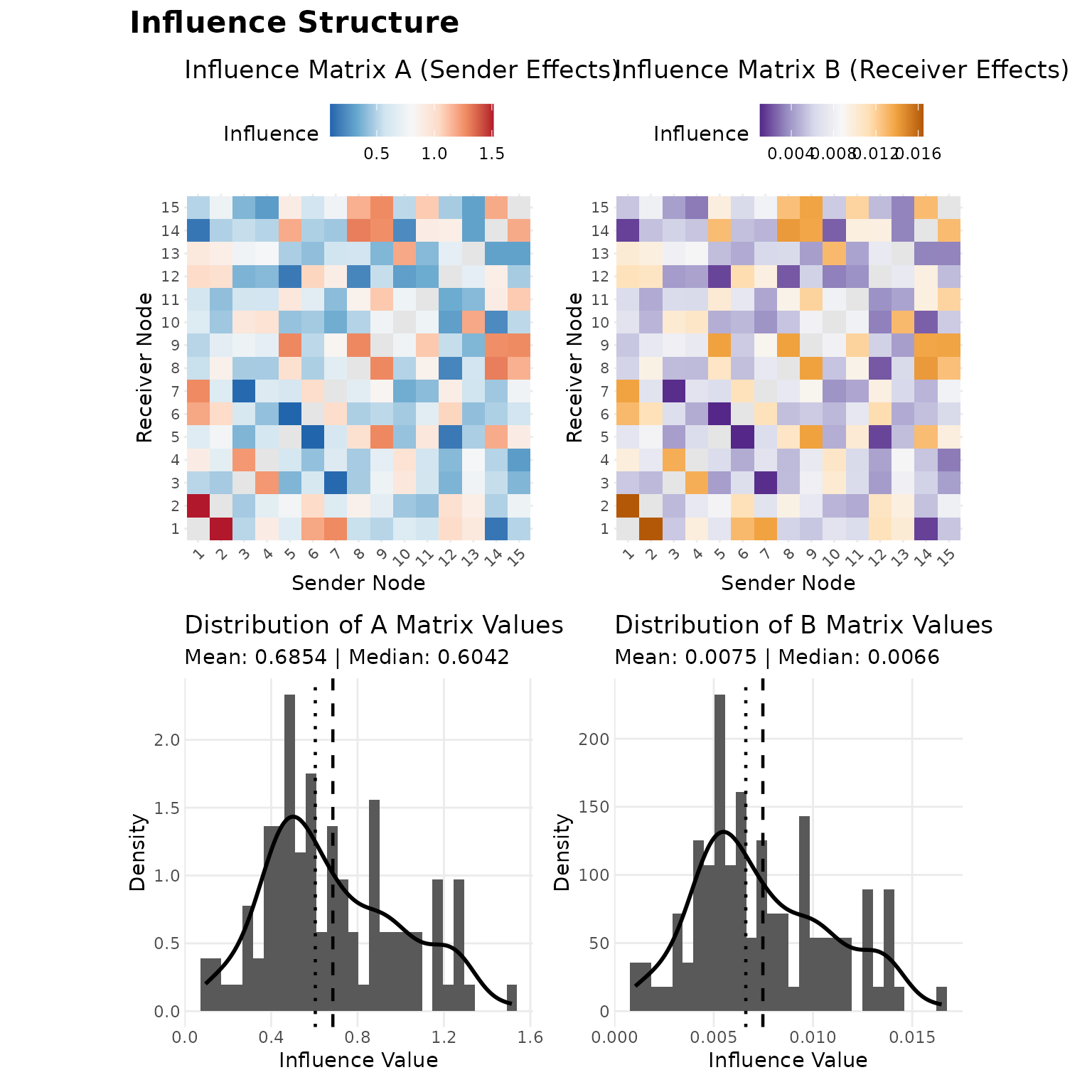

The convergence trace (panel 5) confirms that ALS has stabilized:

plot(fit, which = 5, combine = FALSE)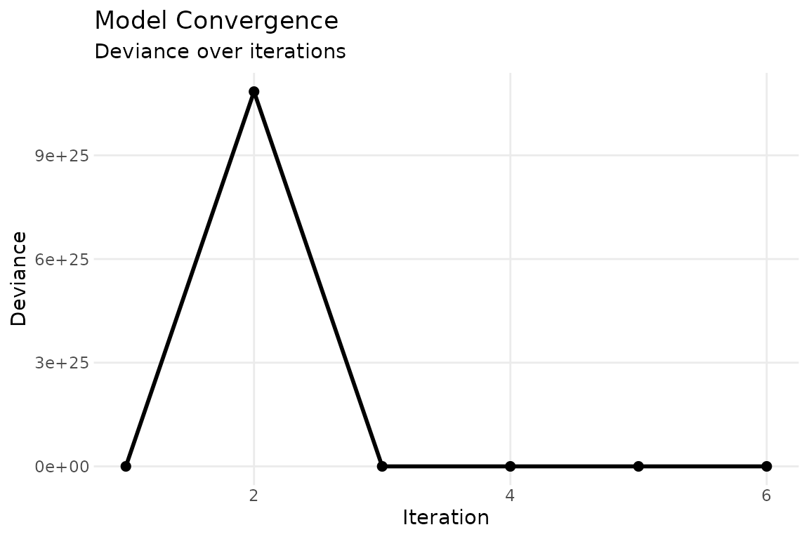

The coefficient plot (panel 6) visualizes parameter estimates with confidence intervals:

plot(fit, which = 6, combine = FALSE)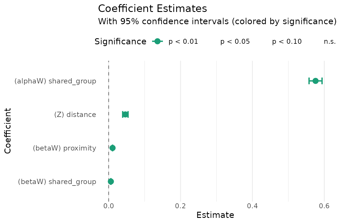

Prediction

predict() returns fitted values on either the link or response scale:

pred = predict(fit, type = "response")

# compare predicted vs observed for a single time slice
obs = Y[,,5]
pred_t5 = pred[,,5]
mask = !is.na(obs)
cor(c(obs[mask]), c(pred_t5[mask]))
#> [1] 0.02298132

For out-of-sample prediction, pass new data via the newdata argument:

predict(fit, newdata = list(Y = Y_new, W = W, X = X_new, Z = Z_new),
    type = "response")

Data format

The package expects data as multidimensional arrays:

Array	Dimensions	Description
`Y`	$m \times m \times T$	Network outcomes (counts, continuous, or binary)
`X`	$m \times m \times T$	Network state carrying influence (typically lagged `Y`)
`W`	$m \times m \times p$	Influence covariates parameterizing $\mathbf{A}$ and $\mathbf{B}$
`Z`	$m \times m \times q \times T$	Exogenous dyadic covariates (optional)

Long-format edge lists can be converted with cast_array(), and rel_covar() constructs relational covariates (main, reciprocal, transitive effects) from a base dyadic variable. See vignette("sir_extensions") for details.

Next steps

Methodology: Full mathematical framework, identifiability, estimation algorithms, and guidance on choosing a model configuration.
Inference: Variance-covariance estimation, fixed-receiver models, bootstrap standard errors, and confidence intervals.
Extensions: Normal and binomial families, symmetric and bipartite networks, dynamic (time-varying) influence covariates, and data preparation utilities.

Shahryar Minhas & Peter Hoff

2026-03-11