lame Overview

Cassy Dorff, Shahryar Minhas, and Tosin Salau

2026-07-25

Package Overview

The lame package provides tools for fitting Longitudinal Additive and Multiplicative Effects models to network data observed over time. If you study relationships between actors (countries trading with each other, legislators co-sponsoring bills, students forming friendships across semesters) and you have repeated observations of those relationships, lame is designed for you.

The modeling approach builds on the Additive and Multiplicative Effects (AME) framework developed by Peter Hoff, whose amen package provides the foundational cross-sectional implementation. lame extends that framework with:

• Longitudinal data: panel networks observed across multiple time periods, potentially with actors entering and leaving the sample.
• Dynamic effects: latent positions and baseline activity levels can evolve via AR(1) processes (dynamic_uv and dynamic_ab).
• C++ acceleration: core sampling routines in Rcpp/RcppArmadillo.
• Bipartite networks: two-mode networks (e.g., countries and treaties) with separate latent spaces for row and column nodes.
• ggplot2-based diagnostics: trace_plot, gof_plot, ab_plot, and uv_plot return standard ggplot2 figures you can theme and extend.
• Standard S3 methods: coef(), confint(), fitted(), residuals(), predict(), and simulate() work as you would expect from any R model object.

The package works with netify for data preparation.

Migrating from amen

Both amen and lame export an ame() function; if both packages are attached, a startup message reminds you that unqualified ame(...) calls dispatch to whichever was attached last, so write lame::ame(...) to be explicit. Old amen scripts largely run unchanged – the most common porting fix is family = "nrm" becoming family = "normal" (the short forms are accepted as aliases, with a message), and print = is deprecated in favour of verbose =. The full mapping of argument and output differences lives in the Migration from amen sections of ?ame and ?lame.

Application: Dutch College Friendships

To see how lame works in practice, we analyze the Dutch college friendship network (van de Bunt, van Duijn, and Snijders 1999), a panel of 32 students who arrived as strangers and rated each other’s friendship at seven time points. (We drop the cold-start first wave, when the students barely knew each other and almost no ties exist; six waves remain.) The substantive question is whether students sort by gender, smoking status, and academic program, and whether residual clustering remains once those covariates are absorbed.

The dataset includes:

• Y: directed friendship ratings on a -1 to 4 scale (-1 a negative/troubled relationship, 0 no or uncertain tie, 1-4 increasing friendship). We binarize any positive rating to a tie ((Y > 0) * 1), so the rare -1 ratings fold in with 0 as “no tie”.
• X: three node-level attributes: male, smoker, program.
• We construct three dyadic homophily indicators from the node attributes: same_male, same_smoker, same_program.

library(lame)
library(ggplot2)
set.seed(6886)

data("dutchcollege")

n <- nrow(dutchcollege$Y)
T_all <- dim(dutchcollege$Y)[3]
actor_names <- sprintf("S%02d", seq_len(n))

# binarize and drop the cold-start wave (t = 1 has almost no ties)
Y <- lapply(2:T_all, function(t) {
    Yt <- (dutchcollege$Y[, , t] > 0) * 1
    diag(Yt) <- NA
    rownames(Yt) <- colnames(Yt) <- actor_names
    Yt
})
names(Y) <- paste0("t", 2:T_all)

# nodal covariates passed identically as sender and receiver
X_node <- dutchcollege$X
rownames(X_node) <- actor_names
Xrow <- lapply(seq_along(Y), function(t) X_node)
Xcol <- Xrow

# dyadic homophily indicators
same_male    <- outer(X_node[, "male"],    X_node[, "male"],    "==") * 1
same_smoker  <- outer(X_node[, "smoker"],  X_node[, "smoker"],  "==") * 1
same_program <- outer(X_node[, "program"], X_node[, "program"], "==") * 1
Xdyad_one <- array(0, dim = c(n, n, 3),
                   dimnames = list(actor_names, actor_names,
                                   c("same_male", "same_smoker", "same_program")))
Xdyad_one[, , 1] <- same_male
Xdyad_one[, , 2] <- same_smoker
Xdyad_one[, , 3] <- same_program
Xdyad <- lapply(seq_along(Y), function(t) Xdyad_one)

The friendship network’s average density rises across the panel as students settle in, though the trajectory is not monotone (density bounces between roughly 0.40 and 0.63 across the six waves):

sapply(Y, function(y) round(mean(y, na.rm = TRUE), 2))
#>   t2   t3   t4   t5   t6   t7 
#> 0.40 0.52 0.47 0.49 0.63 0.51

Fitting the Model

We fit a binary probit AME model with sender random effects (rvar), receiver random effects (cvar), dyadic correlation (dcor), and a one-dimensional latent space (R = 1). The random effects capture sender heterogeneity (some students simply nominate more friends) and receiver heterogeneity (some students are nominated more often), while the latent space picks up residual clustering: students who befriend similar people for reasons the observed covariates do not capture. (Why R = 1 and not 2? See the Latent Space section below.)

fit <- lame(
    Y = Y,
    Xdyad = Xdyad,           # dyadic homophily indicators
    Xrow = Xrow,             # sender covariates
    Xcol = Xcol,             # receiver covariates
    family = "binary",       # binary probit model
    rvar = TRUE,             # sender random effects
    cvar = TRUE,             # receiver random effects
    dcor = TRUE,             # dyadic correlation (reciprocity)
    R = 1,                   # 1-D multiplicative latent space
    symmetric = FALSE,       # friendships are directed
    burn = 30,               # short burn-in for this worked example
    nscan = 150,             # compact post-burn-in run for the vignette
    odens = 10,              # thinning -> 15 stored draws
    posterior_opts = list(save_UV = TRUE),  # keep U/V draws: gives
                                            # latent_positions() real
                                            # posterior SDs below
    save_log_lik = TRUE,     # pointwise log-lik: feeds loo() at the end
    verbose = FALSE,
    plot = FALSE
)

Interpreting the Results

summary(fit)
#> 
#> === Longitudinal AME Model Summary ===
#> 
#> Call:
#> [1] "Y ~ dyad(same_male, same_smoker, same_program) + row(male, smoker, program) + col(male, smoker, program) + a[i] + b[j] + rho*e[ji] + U[i,1:1] %*% V[j,1:1], family = 'binary'"
#> 
#> Time periods: 6 
#> Family: binary 
#> Mode: unipartite 
#> 
#> Note: STATIC fit pooled across 6 time periods --
#>   U, V, a, b are time-invariant; per-period predictions vary
#>   only through per-period covariates. For time-varying effects,
#>   refit with dynamic_uv = TRUE and/or dynamic_ab = TRUE.
#> 
#> Regression coefficients:
#> ------------------------
#>                   Estimate StdError z_value p_value CI_lower CI_upper    
#> intercept           -2.842     1.23  -2.311   0.021   -5.257   -1.645   *
#> male_row             0.975    0.381   2.555   0.011    0.315    1.516   *
#> smoker_row          -1.034    0.429  -2.411   0.016   -1.676   -0.307   *
#> program_row           0.46    0.259   1.772   0.076    0.175    1.013   .
#> male_col             1.089    0.219    4.96       0    0.628    1.389 ***
#> smoker_col           0.015     0.19    0.08   0.936   -0.261    0.351    
#> program_col          0.159    0.148   1.074   0.283   -0.076    0.381    
#> same_male_dyad       0.479    0.057   8.444       0    0.381    0.566 ***
#> same_smoker_dyad     0.183    0.044   4.213       0    0.112    0.248 ***
#> same_program_dyad    0.571    0.061   9.369       0    0.475    0.669 ***
#> ---
#> Signif. codes: 0 '***' 0.001 '**' 0.01 '*' 0.05 '.' 0.1 ' ' 1
#> Note: stars are a visual hint from posterior mean / SD only; for inference use the credible intervals.
#> 
#> Variance components:
#> -------------------
#>     Estimate StdError
#> va     0.867    0.249
#> cab    0.290    0.096
#> vb     0.322    0.083
#> rho    0.325    0.036
#> ve     1.000    0.000
#>   (va = sender, cab = sender-receiver covariance, vb = receiver,
#>    rho = dyadic correlation, ve = residual variance)

A lot lands at once, so let’s walk through it.

Intercept. The probit intercept is the latent linear predictor when every covariate is zero. The covariates here are uncentered (program is coded 2-4 and is never zero), so that corner sits well outside the observed data; the familiar qnorm(density) rule of thumb instead describes the predictor at the average covariate profile. The two reconcile once you add back the mean covariate contribution:

bhat        <- colMeans(fit$BETA)
slice_means <- apply(fit$X[[1]], 3, mean, na.rm = TRUE)   # mean of each design column
centroid_lp <- sum(bhat * slice_means[names(bhat)])       # predictor at the average profile
c(intercept     = unname(bhat["intercept"]),
  centroid_lp   = centroid_lp,
  qnorm_density = qnorm(mean(unlist(Y), na.rm = TRUE)))
#>     intercept   centroid_lp qnorm_density 
#>   -2.84155897   -0.07779080    0.00842291

The intercept itself is strongly negative, but the predictor at the average covariate profile (centroid_lp) sits close to qnorm(density) – the uncentered covariates account for nearly the entire gap. The intercept absorbs the mean covariate contribution; it is not a baseline probability. Center the covariates if you want it to read as one, and read predicted probabilities off predict(fit, type = "response").

Homophily. The three dyadic coefficients (same_male, same_smoker, same_program) measure whether students of the same type are more likely to be friends, holding the sender, receiver, and latent positions fixed. Positive values mean homophily; credible intervals that exclude zero indicate that the direction of the association is well-identified. Program homophily tends to be the strongest of the three, consistent with students bonding around shared coursework.

Nodal covariates. male_row / male_col measure whether male students are unusually active senders or popular receivers, and similarly for smoker and program. With only 32 students, the credible intervals on individual nodal effects are wide; treat the sign as suggestive, the magnitude with caution.

Variance components. va (sender variance) and vb (receiver variance) quantify how much students differ in sociability and popularity beyond what the covariates explain. The dyadic correlation rho captures reciprocity; in friendship networks rho > 0 is the rule rather than the exception.

Checking Convergence

The model is estimated via MCMC, so convergence checks come first. trace_plot shows the sampled values over iterations (top panels) and the corresponding posterior densities (bottom panels) for each parameter.

trace_plot(fit, params = "beta")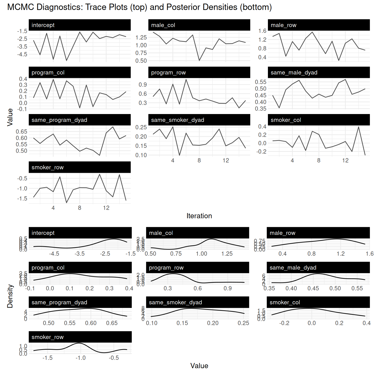

Trace plots should bounce around a stable mean without long-term trends or sticky regions, and density plots should be smooth and unimodal. Numerically, common MCMC checks are split-$\hat R$ < 1.01 for monitored parameters and bulk / tail ESS $\ge$ 400 per chain.

With 15 stored samples, this run cannot meet those thresholds: the number of stored draws caps the ESS, and several $\hat R$ values in the summarise_draws table below land well above 1.01. Read the table as a demonstration of how to check these diagnostics, not as evidence of convergence – for a real analysis, lengthen the chain (burn in the hundreds, nscan in the thousands) until every monitored parameter clears both thresholds. Which parameter mixes worst is seed-dependent in a short chain, so treat this fit as a compact worked example rather than a final diagnostic run.

Bayesian-ecosystem diagnostics: posterior::as_draws()

lame registers as_draws() methods so any fit drops straight into the Stan-era diagnostic ecosystem (posterior, bayesplot, tidybayes): posterior::summarise_draws() gives per-parameter posterior summaries, split-$\hat R$, and bulk / tail ESS in one call.

library(posterior)
#> This is posterior version 1.7.0
#> 
#> Attaching package: 'posterior'
#> The following object is masked from 'package:lame':
#> 
#>     as_draws
#> The following objects are masked from 'package:stats':
#> 
#>     mad, sd, var
#> The following objects are masked from 'package:base':
#> 
#>     %in%, match
draws <- posterior::as_draws(fit)              # draws_array [iter, chain, var]
posterior::summarise_draws(draws)              # rhat, ess_bulk, ess_tail per param
#> Warning: The ESS has been capped to avoid unstable estimates.
#> Warning: The ESS has been capped to avoid unstable estimates.
#> Warning: The ESS has been capped to avoid unstable estimates.
#> Warning: The ESS has been capped to avoid unstable estimates.
#> Warning: The ESS has been capped to avoid unstable estimates.
#> Warning: The ESS has been capped to avoid unstable estimates.
#> Warning: The ESS has been capped to avoid unstable estimates.
#> Warning: The ESS has been capped to avoid unstable estimates.
#> Warning: The ESS has been capped to avoid unstable estimates.
#> Warning: The ESS has been capped to avoid unstable estimates.
#> Warning: The ESS has been capped to avoid unstable estimates.
#> Warning: The ESS has been capped to avoid unstable estimates.
#> Warning: The ESS has been capped to avoid unstable estimates.
#> Warning: The ESS has been capped to avoid unstable estimates.
#> Warning: The ESS has been capped to avoid unstable estimates.
#> Warning: The ESS has been capped to avoid unstable estimates.
#> Warning: The ESS has been capped to avoid unstable estimates.
#> Warning: The ESS has been capped to avoid unstable estimates.
#> Warning: The ESS has been capped to avoid unstable estimates.
#> Warning: The ESS has been capped to avoid unstable estimates.
#> Warning: The ESS has been capped to avoid unstable estimates.
#> Warning: The ESS has been capped to avoid unstable estimates.
#> Warning: The ESS has been capped to avoid unstable estimates.
#> Warning: The ESS has been capped to avoid unstable estimates.
#> Warning: The ESS has been capped to avoid unstable estimates.
#> Warning: The ESS has been capped to avoid unstable estimates.
#> Warning: The ESS has been capped to avoid unstable estimates.
#> # A tibble: 15 × 10
#>    variable            mean  median     sd    mad      q5    q95   rhat ess_bulk
#>    <chr>              <dbl>   <dbl>  <dbl>  <dbl>   <dbl>  <dbl>  <dbl>    <dbl>
#>  1 intercept        -2.84   -2.37   1.23   0.827  -5.20   -1.65   1.40     13.0 
#>  2 male_row          0.975   1.05   0.381  0.431   0.383   1.49   1.14      9.86
#>  3 smoker_row       -1.03   -1.05   0.429  0.178  -1.64   -0.313  0.966    16.0 
#>  4 program_row       0.460   0.377  0.259  0.148   0.218   0.958  1.38     16.0 
#>  5 male_col          1.09    1.11   0.219  0.139   0.753   1.36   1.27      7.26
#>  6 smoker_col        0.0152  0.0376 0.190  0.208  -0.229   0.314  1.02     16.0 
#>  7 program_col       0.159   0.138  0.148  0.121  -0.0691  0.373  1.16     16.0 
#>  8 same_male_dyad    0.479   0.474  0.0567 0.0374  0.406   0.564  0.958    12.1 
#>  9 same_smoker_dyad  0.183   0.188  0.0436 0.0502  0.125   0.244  0.962    16.0 
#> 10 same_program_dy…  0.571   0.583  0.0610 0.0665  0.486   0.653  1.25     11.8 
#> 11 va                0.867   0.906  0.249  0.276   0.536   1.22   0.927    16.0 
#> 12 cab               0.290   0.297  0.0964 0.100   0.160   0.437  1.11     10.7 
#> 13 vb                0.322   0.303  0.0832 0.0784  0.229   0.458  1.11     12.7 
#> 14 rho               0.325   0.327  0.0357 0.0381  0.273   0.374  0.968    13.0 
#> 15 ve                1       1      0      0       1       1     NA        NA   
#> # ℹ 1 more variable: ess_tail <dbl>

A single-chain fit like this one has chain = 1, so $\hat R$ reduces to within-chain split-$\hat R$; for $\hat R$ across independently initialised chains, see the multi-chain section in the dynamic-effects vignette.

Goodness of Fit

The gof_plot function compares observed network statistics to their posterior predictive distributions: can the model reproduce emergent structural features like degree heterogeneity, transitivity, and reciprocity, not just the dyad-level relationships?

gof_plot(fit)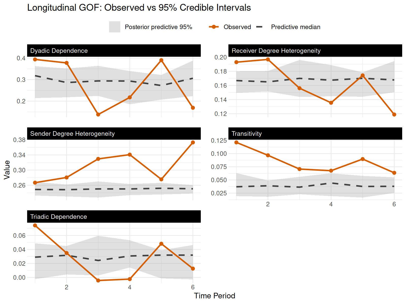

For a longitudinal model, gof_plot shows these statistics across time, encoding three series per panel with colour and linetype redundantly: the observed series is a solid orange line with filled orange points, the posterior-predictive median is a dashed dark line, and the 95% credible interval is a grey ribbon (width set by credible.level). Observed values inside the ribbon are features the model reproduces; values outside flag structure it is missing – itself a substantive finding, not a failure to report.

Reading the figure: the fit comes closest on the cyclic-triad structure (Triadic Dependence sits inside the band at four of the six periods) but under-predicts sender degree heterogeneity (observed above the band at every period) and transitivity (above the band at five of six periods) – some students nominate many more friends than the additive $a_i$ plus latent $u_i$ can absorb, and triangle closure is systematically too low. Receiver heterogeneity drifts in and out of the band across the panel, while Dyadic Dependence (reciprocity) swings from one side of it to the other without settling inside.

This is the standard signature of a latent-space model on a friendship network. AME assumes conditional dyadic independence, so triangle closure must be soaked up by clustering of the latent positions; ERGMs model it directly via terms like gwesp. The two classes are complementary: ERGM for triangle-closure questions, AME for stable, non-degenerate estimates with explicit actor heterogeneity and a coherent posterior to forecast or simulate from.

Posterior-predictive temporal-trend test: gof_temporal()

The figure read above is qualitative. gof_temporal() gives a scalar check on the temporal trend in a chosen statistic: it fits an OLS slope to the observed per-period series, recomputes that slope in posterior-predictive replicate panels drawn via simulate(fit), and returns a two-sided posterior-predictive p-value – near 0 when the observed slope is unreachable under the model, well away from 0 when it is central in the predictive distribution.

# density rises across the panel on net (the network gets denser as
# students settle in, though the trajectory is not monotone), so it is the
# natural temporal-trend target.
gt_density <- gof_temporal(fit, stat = "density", n_rep = 100, seed = 6886)
gt_density   # prints stat, observed slope, n_rep, and the p_pp
#> 
#> ── Temporal-trend posterior-predictive check ──
#> 
#> • Statistic: "density"
#> • Observed slope (per-period): 0.025
#> • Replicates: 100
#> • Posterior-predictive p-value (two-sided): 0
#> Observed temporal trend is incompatible with the fitted model.

A p_pp of 0 says the static fit cannot reproduce the empirical net densification slope (about +0.025 per period in our run) – the expected diagnostic for a model whose parameters are constant across periods, and consistent with the per-period mass shift in gof_plot(). dynamic_beta or time-varying covariates are the remedy; see the Dynamic Effects vignette.

Latent Space

The multiplicative effects capture association patterns beyond what the covariates and additive effects explain. We fit R = 1, so each student’s sender position ($u_i$) and receiver position ($v_i$) is a single number – and a one-dimensional space should be plotted as one dimension (a 2-D scatter of a 1-D space piles every point onto a line and looks degenerate even when the positions are informative). Why not just fit R = 2? Extra dimensions are not free: they can absorb signal the dyadic covariates would otherwise pick up, and a one-dimensional space is far easier to display and interpret. Parsimony wins here; to let the data adjudicate a rank choice, compare fits with loo::loo_compare() out of sample, as done for R = 1 versus R = 0 at the end of this vignette.

The honest display for a 1-D space is a ranked dot plot: every student’s sender and receiver position with a 95% interval, ordered by sender position. The intervals come from the saved U/V draws (posterior_opts = list(save_UV = TRUE) in the fit above).

lp1 <- subset(latent_positions(fit), dimension == 1)
ordv <- with(subset(lp1, type == "U"), actor[order(value)])
lp1$actor <- factor(lp1$actor, levels = ordv)

ggplot(lp1, aes(x = value, y = actor, color = type)) +
    geom_vline(xintercept = 0, linetype = 2, color = "grey60") +
    geom_errorbar(aes(xmin = value - 2 * posterior_sd,
                      xmax = value + 2 * posterior_sd),
                  width = 0, alpha = 0.5, orientation = "y") +
    geom_point(size = 1.8) +
    scale_color_manual(values = c(U = "#D55E00", V = "#0072B2"),
                       labels = c(U = "sender (u)", V = "receiver (v)")) +
    labs(x = "Latent position (dimension 1)", y = NULL, color = NULL) +
    theme_bw() +
    theme(panel.border = element_blank(), panel.grid.major.y = element_blank(),
          axis.ticks = element_blank(), legend.position = "top")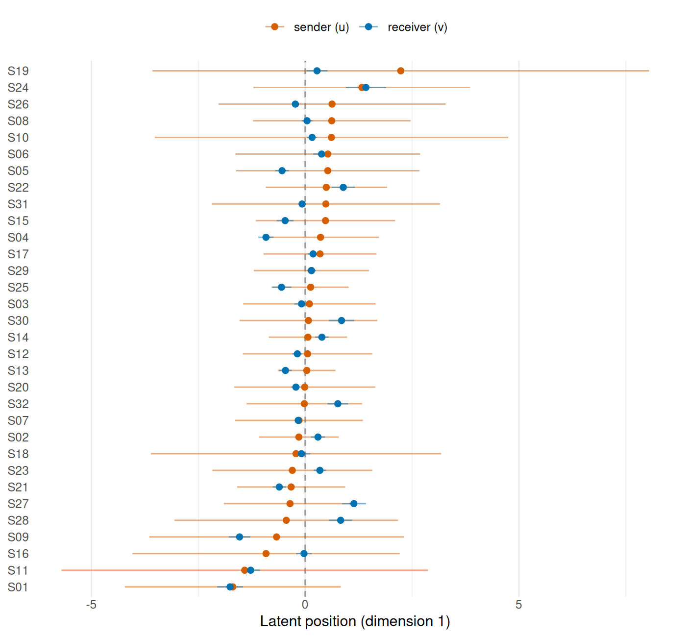

Three things to read off this plot. First, the dimension is genuinely informative: the extremes (around $+1.7$ at the top versus $-1.1$ at the bottom) are separated by roughly twice the width of a typical 95% interval, so the ordering is signal, not noise. Second, sender and receiver positions are strongly related (their correlation is about 0.55): students near the top both seek out and attract the same friendship cluster. Third, the exceptions are the interesting actors – students whose blue and orange points diverge are attractive to a cluster they do not themselves reach toward (or vice versa), a pattern no covariate in the model encodes. These static positions are pooled across all six waves; if you suspect students moved through this space as the year progressed, that is what dynamic_uv = TRUE estimates (see the dynamic effects vignette).

Extracting Latent Positions

If you need the estimated latent positions in a tidy format (for custom plots, merging with external data, or exporting to other tools), the latent_positions() function returns a data frame:

lp <- latent_positions(fit)
head(lp)
#>   actor dimension time       value posterior_sd type
#> 1   S01         1    1 -1.69217879    1.2629097    U
#> 2   S02         1    1 -0.14694728    0.4667172    U
#> 3   S03         1    1  0.09914408    0.7743679    U
#> 4   S04         1    1  0.35976832    0.6822472    U
#> 5   S05         1    1  0.52953437    1.0736528    U
#> 6   S06         1    1  0.53141713    1.0800417    U

Each row gives one actor’s position on one latent dimension at one time point, with a type column distinguishing the sender position ("U") from the receiver position ("V"). The posterior_sd column is populated because the fit saved its U/V draws (posterior_opts = list(save_UV = TRUE)); without that option it is NA with a one-time message telling you how to refit. A static fit returns a single slice (labelled time = 1) that applies to every period; dynamic fits (dynamic_uv = TRUE) return each time point separately, and procrustes_align() removes the arbitrary per-period rotations so that trajectories across time are interpretable (see the dynamic effects vignette).

Tidy-data round-trip via netify

lame uses the netify package for tidy network data: build a netify object from an edgelist and pass it directly to lame() or ame(). On the way out, tidy(), autoplot(), and prediction_draws_long() give you broom-/ggplot-/marginaleffects-ready output.

Entry: tidy edgelist → lame()

library(netify)

# a tidy edgelist is often how network data arrives. Here we melt the
# Dutch-college wave list back into one (from, to, year, tie) row per
# ordered dyad, carrying a dyadic covariate along for the ride.
edges_long <- do.call(rbind, lapply(seq_along(Y), function(t) {
    Yt  <- Y[[t]]
    idx <- which(!is.na(Yt), arr.ind = TRUE)
    data.frame(
        from = rownames(Yt)[idx[, 1]],
        to   = colnames(Yt)[idx[, 2]],
        year = names(Y)[t],
        tie  = as.integer(Yt[idx]),
        same_program = Xdyad[[t]][, , "same_program"][idx]
    )
}))
head(edges_long)
#>   from  to year tie same_program
#> 1  S02 S01   t2   0            0
#> 2  S03 S01   t2   0            0
#> 3  S04 S01   t2   0            0
#> 4  S05 S01   t2   0            0
#> 5  S06 S01   t2   0            0
#> 6  S07 S01   t2   1            0

netlet <- netify::netify(
    edges_long,
    actor1 = "from", actor2 = "to", time = "year",
    weight = "tie", dyad_vars = "same_program",
    symmetric = FALSE, mode = "unipartite",
    missing_to_zero = FALSE,
    output_format = "longit_array"
)

# a netify object drops straight into lame(); reduced iterations here so the
# vignette builds quickly (use burn >= 500, nscan >= 4000 for real analyses).
fit_netlet <- lame(
    netlet,
    family = "binary", R = 1,
    burn = 50, nscan = 200, odens = 5,
    verbose = FALSE
)

# to inspect what lame() will see, to_lame() returns the pieces directly
pieces <- netify::to_lame(netlet, lame = TRUE)
names(pieces)
#> [1] "Y"          "Xdyad"      "Xrow"       "Xcol"       "mode"      
#> [6] "family"     "ame_call"   "fit_method" "bootstrap"

fit_netlet is a live fit taken straight off the netify object – no reshaping, no hand-built lists – and names(pieces) shows the inputs lame() actually consumes (Y, Xdyad, Xrow, Xcol, plus the mode / family metadata netify carries). The payoff is the alignment: netify() rebuilt, for every period, a tie matrix and a covariate slice keyed to the same actor order – exactly the rownames-and-array() bookkeeping done by hand in the setup chunk at the top of this vignette. When your data arrives as an edgelist, as panel network data usually does, the edgelist is the only object you touch.

Exit: tidy(), autoplot(), prediction_draws_long()

The rest of the round-trip runs against the fit object built from the Dutch-college data above:

# tidy(fit) -> term / estimate / std.error / statistic / p.value /
# conf.low / conf.high; one row per coefficient (or per
# coefficient x period for dynamic_beta fits). The generic ships with
# lame so this runs without broom installed; when broom is on the path
# `broom::tidy(fit)` dispatches to the same method via
# generics::tidy registration.
tidy(fit)
#> # A tibble: 10 × 7
#>    term              estimate std.error statistic     p.value conf.low conf.high
#>    <chr>                <dbl>     <dbl>     <dbl>       <dbl>    <dbl>     <dbl>
#>  1 intercept          -2.84      1.23     -2.31   0.0208       -5.26      -1.64 
#>  2 male_row            0.975     0.381     2.55   0.0106        0.315      1.52 
#>  3 smoker_row         -1.03      0.429    -2.41   0.0159       -1.68      -0.307
#>  4 program_row         0.460     0.259     1.77   0.0764        0.175      1.01 
#>  5 male_col            1.09      0.219     4.96   0.000000704   0.628      1.39 
#>  6 smoker_col          0.0152    0.190     0.0802 0.936        -0.261      0.351
#>  7 program_col         0.159     0.148     1.07   0.283        -0.0762     0.381
#>  8 same_male_dyad      0.479     0.0567    8.44   0             0.381      0.566
#>  9 same_smoker_dyad    0.183     0.0436    4.21   0.0000252     0.112      0.248
#> 10 same_program_dyad   0.571     0.0610    9.37   0             0.475      0.669

Coefficient tables: glance() + tidy() -> modelsummary / gt / kableExtra

Because tidy() and glance() are registered against their generics counterparts, any broom-aware table package consumes a lame fit directly – most compactly modelsummary::modelsummary(fit):

# glance() returns the one-row model summary modelsummary uses for its
# lower panel: nobs, n_actors, n_periods, n_stored, family, mode, R,
# dynamic_uv / dynamic_ab / dynamic_beta, elpd_loo (NA unless save_log_lik=TRUE).
broom::glance(fit)
#> # A tibble: 1 × 13
#>    nobs n_actors n_row_actors n_col_actors n_periods n_stored family mode      R
#>   <int>    <int>        <int>        <int>     <int>    <int> <chr>  <chr> <int>
#> 1  5952       32           NA           NA         6       15 binary unip…     1
#> # ℹ 4 more variables: dynamic_uv <lgl>, dynamic_ab <lgl>, dynamic_beta <lgl>,
#> #   elpd_loo <dbl>

# pass the fit straight to modelsummary -- tidy() drives the upper
# (coefficients) panel, glance() drives the lower (GOF) panel.
modelsummary::modelsummary(
    list("Dutch college" = fit),
    statistic = "conf.int",
    gof_map = c("nobs", "n_actors", "n_periods", "n_stored",
                "family", "R", "dynamic_uv", "dynamic_ab")
)

	Dutch college
intercept	-2.842
	[-5.257, -1.645]
male_row	0.975
	[0.315, 1.516]
smoker_row	-1.034
	[-1.676, -0.307]
program_row	0.460
	[0.175, 1.013]
male_col	1.089
	[0.628, 1.389]
smoker_col	0.015
	[-0.261, 0.351]
program_col	0.159
	[-0.076, 0.381]
same_male_dyad	0.479
	[0.381, 0.566]
same_smoker_dyad	0.183
	[0.112, 0.248]
same_program_dyad	0.571
	[0.475, 0.669]
Num.Obs.	5952
n_actors	32
n_periods	6
n_stored	15
family	binary
R	1
dynamic_uv	FALSE
dynamic_ab	FALSE

Multiple fits compose into a side-by-side table via a named list, one column per fit. Below we compare the full specification against a no-latent-space variant (R = 0):

fit_noUV <- lame(
    Y = Y, Xdyad = Xdyad, Xrow = Xrow, Xcol = Xcol,
    family = "binary", rvar = TRUE, cvar = TRUE, dcor = TRUE,
    R = 0,                          # no latent space
    symmetric = FALSE,
    burn = 30, nscan = 150, odens = 10,
    save_log_lik = TRUE,            # reused by loo_compare() below
    verbose = FALSE, plot = FALSE
)

modelsummary::modelsummary(
    list("AME (R = 1)" = fit, "Additive only (R = 0)" = fit_noUV),
    statistic = "conf.int",
    gof_map = c("nobs", "n_actors", "n_periods", "n_stored",
                "family", "R", "dynamic_uv", "dynamic_ab")
)

	AME (R = 1)	Additive only (R = 0)
intercept	-2.842	-1.937
	[-5.257, -1.645]	[-3.444, -0.836]
male_row	0.975	0.720
	[0.315, 1.516]	[0.051, 1.473]
smoker_row	-1.034	-0.939
	[-1.676, -0.307]	[-1.618, -0.371]
program_row	0.460	0.316
	[0.175, 1.013]	[0.082, 0.553]
male_col	1.089	0.967
	[0.628, 1.389]	[0.585, 1.242]
smoker_col	0.015	-0.137
	[-0.261, 0.351]	[-0.586, 0.325]
program_col	0.159	0.080
	[-0.076, 0.381]	[-0.127, 0.331]
same_male_dyad	0.479	0.432
	[0.381, 0.566]	[0.340, 0.500]
same_smoker_dyad	0.183	0.190
	[0.112, 0.248]	[0.103, 0.259]
same_program_dyad	0.571	0.622
	[0.475, 0.669]	[0.537, 0.696]
Num.Obs.	5952	5952
n_actors	32	32
n_periods	6	6
n_stored	15	15
family	binary	binary
R	1	0
dynamic_uv	FALSE	FALSE
dynamic_ab	FALSE	FALSE

Reading down the two columns shows how a latent space can redistribute signal: when residual clustering is real, homophily coefficients move toward zero in the AME column because structure that was loaded onto same_program (etc.) is instead absorbed by the latent positions. On this small panel the movement is modest, with widely overlapping credible intervals – the direction is what to look for, not the exact shift.

# autoplot.lame returns a horizontal coefplot for static fits and a
# ribbon-per-period for dynamic_beta fits, so the same call works for
# both. ggplot layers compose on top.
autoplot(fit) +
    ggtitle("Dutch college friendship: posterior coefficients")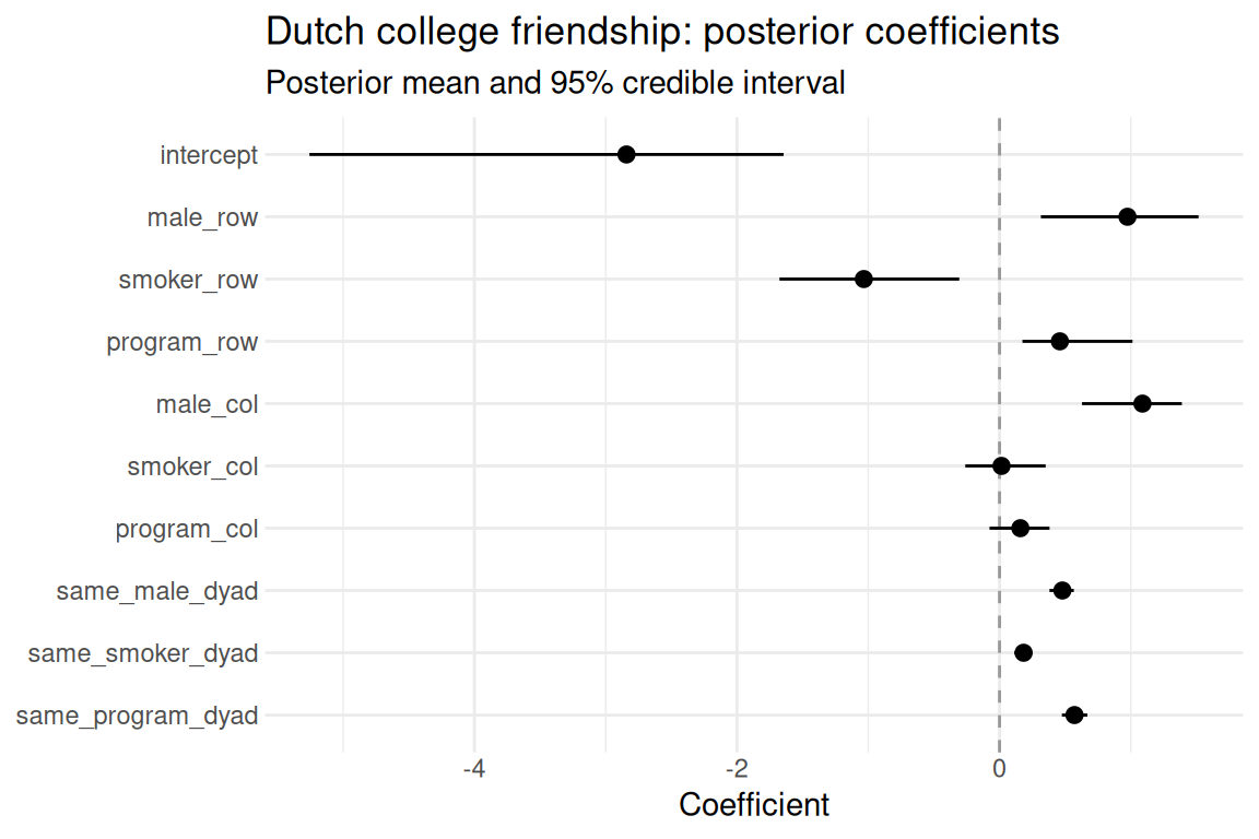

The coefplot is the visual form of the tidy(fit) table above: the three homophily terms sit clear of the dashed zero line – same_program largest (0.57), same_male next (0.45), same_smoker smallest (0.16) – while the nodal terms are mixed, with smoker_col and program_col straddling the line. The same generic dispatches on which = "uv" (latent positions – the ranked dot plot in the Latent Space section above) and which = "ab" (sender / receiver random effects):

# which = "ab" delegates to ab_plot() (sender side by default; use
# ab_plot(fit, effect = "receiver") for the column side). Each lollipop
# is a student's sender random effect a_i: the longest positive stems
# are students who nominate far more friends than their covariates
# predict -- the heterogeneity that va summarises as one number.
autoplot(fit, which = "ab")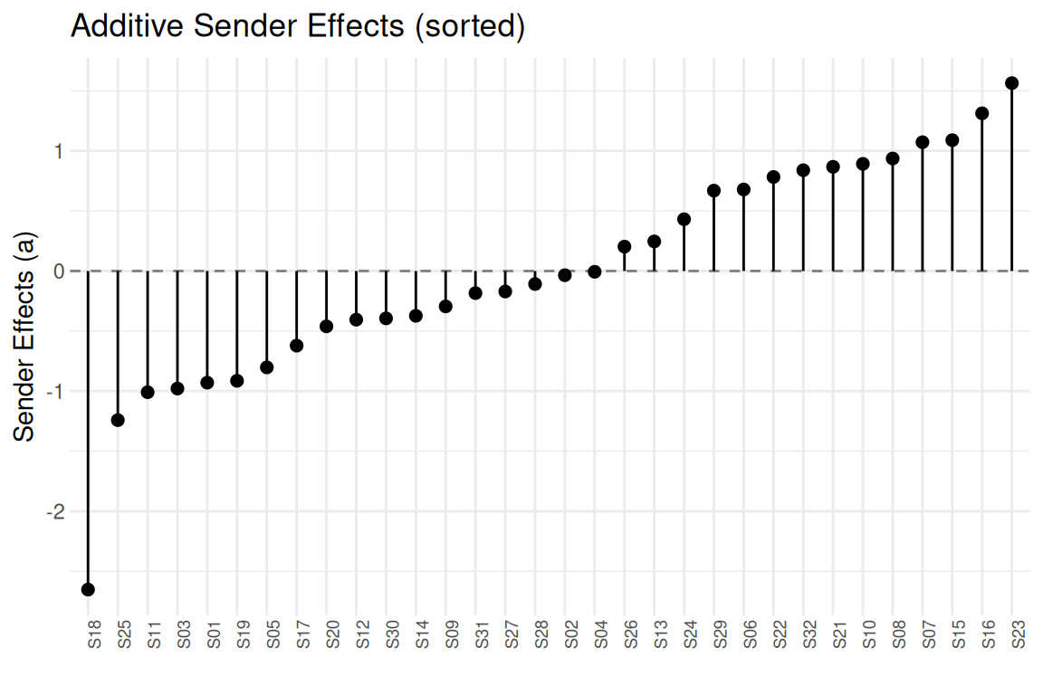

# prediction_draws_long() returns a long-format data frame with
# .chain / .iteration / .draw / period / period_label / i / j /
# actor_i / actor_j / .value -- ready for tidybayes / marginaleffects.
pdl <- prediction_draws_long(fit, type = "response", n_draws = 50)
# the diagonal (i == j) is a self-tie, undefined in a friendship network, but
# the linear predictor is still numerically defined there -- drop it so the
# frame covers only real (off-diagonal) pairs.
pdl <- pdl[pdl$i != pdl$j, ]
head(pdl, 3)
#> # A tibble: 3 × 10
#>   .chain .iteration .draw period period_label     i     j actor_i actor_j
#>    <int>      <int> <int>  <int> <chr>        <int> <int> <chr>   <chr>  
#> 1      1          1     1      1 t2               2     1 S02     S01    
#> 2      1          1     1      1 t2               3     1 S03     S01    
#> 3      1          1     1      1 t2               4     1 S04     S01    
#> # ℹ 1 more variable: .value <dbl>
dim(pdl)
#> [1] 297600     10

Because the .chain / .iteration / .draw / .value columns follow the tidybayes / marginaleffects convention, this frame composes directly with ggdist, tidybayes, and marginaleffects – no reshaping step needed.

Model comparison: loo::loo_compare() as a one-liner

Does the latent space earn its keep over additive effects alone? The standard out-of-sample yardstick is the expected log pointwise predictive density (elpd_loo) from loo::loo(), which requires save_log_lik = TRUE at fit time; the mechanics (and the Pareto-$k$ diagnostics to read before trusting any elpd number) are covered in Your First AME Model. Both fits above already carry the pointwise log-likelihood, so loo::loo_compare() ranks them in one call:

# both fits already carry save_log_lik = TRUE, so this reuses them -- no
# refitting. Pass a NAMED list so the rows are labelled by model rather
# than model1/model2.
cmp <- loo::loo_compare(list(no_latent = loo::loo(fit_noUV),
                             latent_R1 = loo::loo(fit)))
cmp
#>      model elpd_diff se_diff p_worse diag_diff          diag_elpd
#>  latent_R1       0.0     0.0      NA           5952 k_psis > 0.15
#>  no_latent    -147.2    18.9    1.00           5952 k_psis > 0.15

How to read the output. The top row is the preferred model (elpd_diff = 0); each subsequent row reports the elpd difference relative to it, with a standard error. Here 1 is preferred, beating 2 by about 147.2 elpd units (SE 18.9); a ratio of |elpd_diff|/se_diff near or above 2 is a reasonably confident preference, so the latent space is doing real predictive work on this network. When |elpd_diff| is instead close to its SE, the simpler model is the defensible choice.

This result sits comfortably beside the earlier modelsummary table, where the R = 1 and R = 0 columns told the same homophily story (the nodal terms shift more, with wide overlapping intervals). The two are not in tension: the latent space leaves the homophily coefficients intact yet buys roughly 147.2 elpd units out of sample, because the predictive gain is carried by the estimated latent positions themselves – the $u_i' v_j$ term in the linear predictor. Residual dyadic structure shows up in held-out predictive density long before it shows up in a coefficient table.

Reproducibility: sessionInfo() and renv.lock

An analysis a reviewer (or your future self) can reproduce records the seed and the package versions it was fit under. The pattern:

fit <- lame(..., seed = 6886)          # the sampler seed lives in lame()
saveRDS(list(fit = fit, session = sessionInfo()),
        file = "lame_fit_replication.rds")

For long-term reproducibility, commit an renv.lock so reviewers can recreate the toolchain with renv::restore(). This vignette’s own session record:

sessionInfo()
#> R version 4.6.1 (2026-06-24)
#> Platform: x86_64-pc-linux-gnu
#> Running under: Ubuntu 24.04.4 LTS
#> 
#> Matrix products: default
#> BLAS:   /usr/lib/x86_64-linux-gnu/openblas-pthread/libblas.so.3 
#> LAPACK: /usr/lib/x86_64-linux-gnu/openblas-pthread/libopenblasp-r0.3.26.so;  LAPACK version 3.12.0
#> 
#> locale:
#>  [1] LC_CTYPE=C.UTF-8       LC_NUMERIC=C           LC_TIME=C.UTF-8       
#>  [4] LC_COLLATE=C.UTF-8     LC_MONETARY=C.UTF-8    LC_MESSAGES=C.UTF-8   
#>  [7] LC_PAPER=C.UTF-8       LC_NAME=C              LC_ADDRESS=C          
#> [10] LC_TELEPHONE=C         LC_MEASUREMENT=C.UTF-8 LC_IDENTIFICATION=C   
#> 
#> time zone: UTC
#> tzcode source: system (glibc)
#> 
#> attached base packages:
#> [1] stats     graphics  grDevices utils     datasets  methods   base     
#> 
#> other attached packages:
#> [1] netify_1.5.3    posterior_1.7.0 ggplot2_4.0.3   lame_1.3.5     
#> 
#> loaded via a namespace (and not attached):
#>  [1] gtable_0.3.6          tensorA_0.36.2.1      xfun_0.60            
#>  [4] bslib_0.11.0          bayestestR_0.18.1     insight_1.5.2        
#>  [7] ggrepel_0.9.8         lattice_0.22-9        vctrs_0.7.3          
#> [10] tools_4.6.1           generics_0.1.4        datawizard_1.3.1     
#> [13] parallel_4.6.1        tibble_3.3.1          pkgconfig_2.0.3      
#> [16] tinytable_0.17.0      data.table_1.18.4     checkmate_2.3.4      
#> [19] ggnewscale_0.5.2      RColorBrewer_1.1-3    S7_0.2.2             
#> [22] desc_1.4.3            distributional_0.8.1  lifecycle_1.0.5      
#> [25] compiler_4.6.1        farver_2.1.2          textshaping_1.0.5    
#> [28] htmltools_0.5.9       sass_0.4.10           yaml_2.3.12          
#> [31] pillar_1.11.1         pkgdown_2.2.1         jquerylib_0.1.4      
#> [34] tidyr_1.3.2           cachem_1.1.0          abind_1.4-8          
#> [37] network_1.20.0        tidyselect_1.2.1      digest_0.6.39        
#> [40] performance_0.17.1    dplyr_1.2.1           purrr_1.2.2          
#> [43] labeling_0.4.3        fastmap_1.2.0         grid_4.6.1           
#> [46] cli_3.6.6             magrittr_2.0.5        patchwork_1.3.2      
#> [49] loo_2.10.1            utf8_1.2.6            broom_1.0.13         
#> [52] withr_3.0.3           scales_1.4.0          backports_1.5.1      
#> [55] rmarkdown_2.31        matrixStats_1.5.0     igraph_2.3.3         
#> [58] otel_0.2.0            modelsummary_2.6.0    ragg_1.5.2           
#> [61] coda_0.19-4.1         evaluate_1.0.5        knitr_1.51           
#> [64] parameters_0.29.2     rlang_1.3.0           Rcpp_1.1.2           
#> [67] glue_1.8.1            jsonlite_2.0.0        R6_2.6.1             
#> [70] statnet.common_4.13.0 tables_0.9.35         systemfonts_1.3.2    
#> [73] fs_2.1.0

What’s Next?

This vignette covered the core workflow: fitting, convergence, GOF, and visualization. For more specialized topics:

• Single networks (no time series)? See Your First AME Model for a detailed cross-sectional walkthrough
• Two types of nodes? See Bipartite Networks
• Evolving network structure? See Dynamic Effects
• Just want the quick version? See Getting Started

References:

Hoff, PD (2021) Additive and Multiplicative Effects Network Models. Statistical Science 36, 34–50.

van de Bunt, G. G., van Duijn, M. A. J., & Snijders, T. A. B. (1999). Friendship networks through time: An actor-oriented dynamic statistical network model. Computational & Mathematical Organization Theory, 5(2), 167–192.

Minhas, S., Dorff, C., Gallop, M. B., Foster, M., Liu, H., Tellez, J., & Ward, M. D. (2022). Taking dyads seriously. Political Science Research and Methods, 10(4), 703–721. doi:10.1017/psrm.2021.56