Multilayer Networks

This vignette demonstrates how to analyze multilayer networks in netify. Multilayer networks capture multiple types of relationships between the same actors – a crucial feature for understanding complex political systems where actors interact through various channels simultaneously.

Traditional network analysis forces us to choose: study trade OR conflict, cooperation OR competition, formal OR informal ties. But political reality is multilayered. States that trade may also fight. Legislators who cosponsor bills may attack each other on social media. Ignoring these multiple, simultaneous relationships leads to incomplete and potentially misleading conclusions.

Multilayer networks solve this problem by allowing us to analyze multiple relationship types together, revealing:

Substitution effects: Do actors use one type of relationship instead of another?
Complementarities: Do certain relationships tend to co-occur?
Cross-layer influence: Does position in one network affect behavior in another?
Structural coupling: How do different relationship types shape each other?

Quick Start Example

We’ll use data from the Integrated Crisis Early Warning System (ICEWS) throughout here.

library(netify)
library(tidyverse)

# Load the ICEWS event data
data(icews)

# Create a simple multilayer network for 2010
icews_2010 <- icews[icews$year == 2010, ]

# Verbal cooperation network
verbal_net <- netify(
    icews_2010,
    actor1 = "i", actor2 = "j",
    weight = "verbCoop"
)

# Material cooperation network
material_net <- netify(
    icews_2010,
    actor1 = "i", actor2 = "j",
    weight = "matlCoop"
)

# Combine into multilayer network
multi_net <- layer_netify(
    list(verbal = verbal_net, material = material_net)
)

# Quick visualization
plot(multi_net, add_text = FALSE)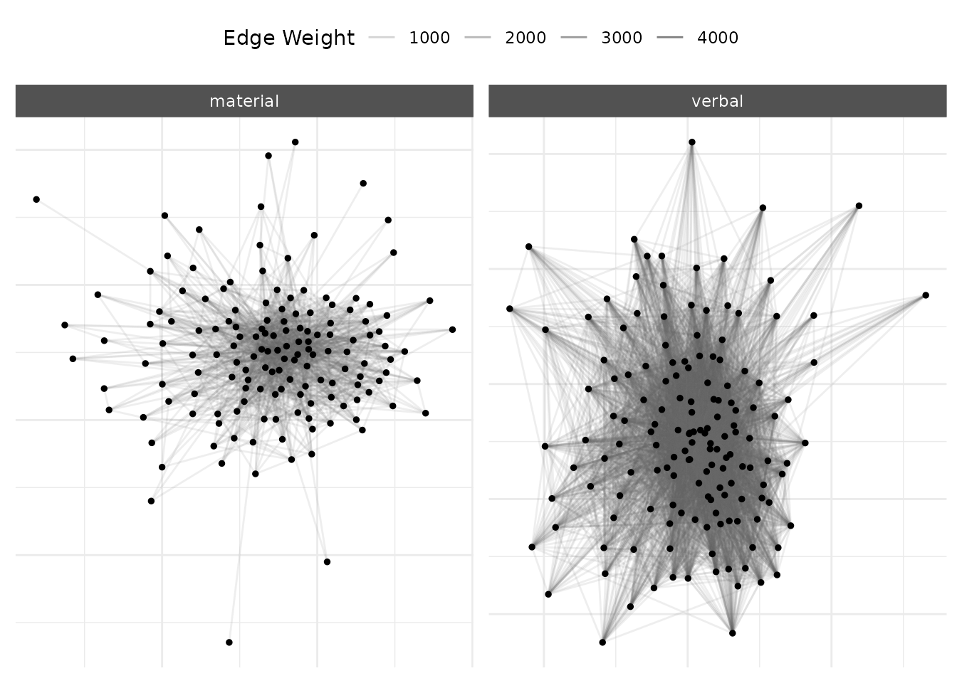

What we see: Even this simple example reveals the “cheap talk” problem in international relations. The verbal cooperation network (left) is dense with connections, while material cooperation (right) is sparse. Most diplomatic promises don’t translate into material support.

Building Multilayer Networks: A Substantive Example

Let’s build a more complete multilayer network to study international cooperation patterns during a critical period – 2002, shortly after 9/11 when cooperation dynamics were rapidly shifting.

# Focus on 2002 - post-9/11 cooperation dynamics
icews_2002 <- icews[icews$year == 2002, ]

# Create networks with relevant attributes
verbal_coop_net <- netify(
    icews_2002,
    actor1 = "i", actor2 = "j",
    symmetric = TRUE,
    weight = "verbCoop",
    nodal_vars = c("i_polity2", "i_log_gdp", "i_log_pop", "i_region"),
    dyad_vars = c("verbConf", "matlConf")
)

material_coop_net <- netify(
    icews_2002,
    actor1 = "i", actor2 = "j",
    symmetric = TRUE,
    weight = "matlCoop",
    nodal_vars = c("i_polity2", "i_log_gdp", "i_log_pop", "i_region"),
    dyad_vars = c("verbConf", "matlConf")
)

# Combine into multilayer network
multilayer_net <- layer_netify(
    netlet_list = list(verbal_coop_net, material_coop_net),
    layer_labels = c("Verbal", "Material")
)

print(multilayer_net)

Visualizing Multilayer Structures

Basic Visualization with Interpretation

plot(multilayer_net,
    add_text = FALSE,
    node_size_by = "i_log_gdp",
    node_color_by = "i_region"
) +
    theme(
        legend.position = "right"
    )

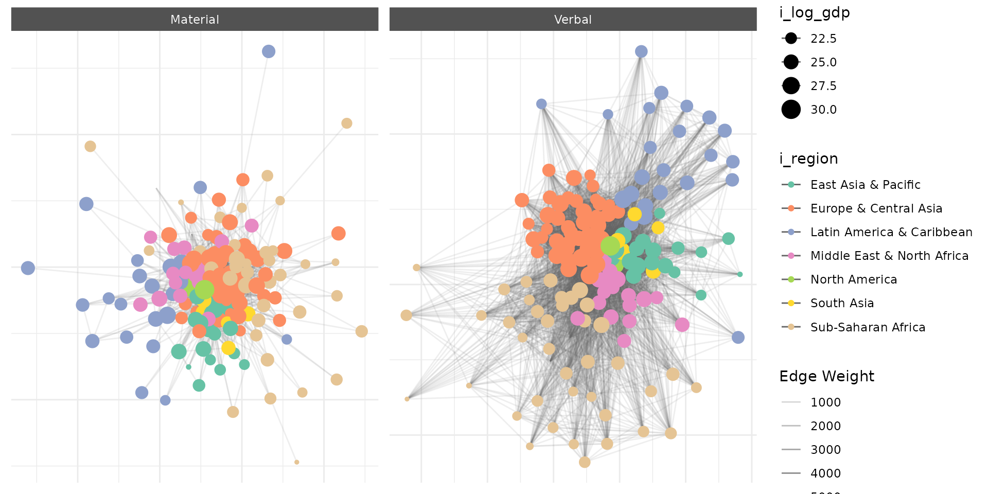
This visualization reveals the fundamental asymmetry in international cooperation. The verbal layer shows the “diplomatic commons” – nearly all countries engage in diplomatic discourse. The material layer reveals the “cooperation core” – a much smaller set of countries that back words with resources. Node sizes (GDP) show that while large economies participate in both networks, material cooperation isn’t simply a function of capacity.

Comparing Network Structures

# Get structural comparison
struct_comp <- compare_networks(multilayer_net, what = "structure")
print(struct_comp)
#>    network n_nodes n_edges   density reciprocity transitivity mean_degree
#> 1   Verbal     152    9378 0.4059037          NA    0.6058952   123.39474
#> 2 Material     152    2576 0.1114958          NA    0.3106440    33.89474
#>   centralization
#> 1     0.03999949
#> 2     0.03794829
#>                        metric   value_net1   value_net2 absolute_change
#> n_nodes               n_nodes 1.520000e+02 1.520000e+02    0.000000e+00
#> n_edges               n_edges 9.378000e+03 2.576000e+03   -6.802000e+03
#> density               density 4.059037e-01 1.114958e-01   -2.944079e-01
#> reciprocity       reciprocity           NA           NA              NA
#> transitivity     transitivity 6.058952e-01 3.106440e-01   -2.952512e-01
#> mean_degree       mean_degree 1.233947e+02 3.389474e+01   -8.950000e+01
#> centralization centralization 3.999949e-02 3.794829e-02   -2.051197e-03
#>                percent_change
#> n_nodes              0.000000
#> n_edges            -72.531457
#> density            -72.531457
#> reciprocity                NA
#> transitivity       -48.729753
#> mean_degree        -72.531457
#> centralization      -5.128059

What these numbers mean:

4x density difference: For every material cooperation relationship, there are four verbal ones
3.6x degree difference: The average country verbally cooperates with 123 others but materially supports only 34
Different clustering: Higher transitivity in verbal cooperation (0.606 vs 0.311) suggests diplomatic communities form more readily than material support clusters

This structural evidence supports the “cheap talk” hypothesis but also reveals something deeper: material cooperation follows different organizational logics than diplomacy.

Testing Political Science Theories with Multilayer Networks

Theory 1: Democratic Peace in Different Domains

Do democracies cooperate more with each other? And does this vary by cooperation type?

# Test homophily across layers
multilayer_homophily <- homophily(
    multilayer_net,
    attribute = "i_polity2",
    method = "correlation"
)

print(multilayer_homophily)
#>   net    layer attribute      method threshold_value homophily_correlation
#> 1   1   Verbal i_polity2 correlation               0            0.04162793
#> 2   1 Material i_polity2 correlation               0            0.01444973
#>   mean_similarity_connected mean_similarity_unconnected similarity_difference
#> 1                 -6.964294                   -7.444698             0.4804043
#> 2                 -7.016653                   -7.279288             0.2626347
#>   p_value     ci_lower   ci_upper n_connected_pairs n_unconnected_pairs
#> 1   0.000  0.022350124 0.06111234              4453                6573
#> 2   0.138 -0.006434521 0.03534843              1201                9825
#>   n_missing n_pairs
#> 1         3   11476
#> 2         3   11476

Democratic homophily exists in verbal cooperation (p < 0.001) but not material cooperation (p = 0.13). This suggests the “democratic peace” operates primarily through diplomatic channels. Material support crosses regime boundaries, likely driven by strategic rather than ideological considerations.

Theory 2: Regional Security Complexes

Do security concerns create regional cooperation clusters? Let’s examine regional patterns:

# Regional mixing patterns
multilayer_mixing <- mixing_matrix(
    multilayer_net,
    attribute = "i_region"
)

print(multilayer_mixing$summary_stats)
#>   net    layer attribute assortativity diagonal_proportion  entropy modularity
#> 1   1   Verbal  i_region     0.1558717           0.3365323 3.350767   0.122512
#> 2   1 Material  i_region     0.2184878           0.3835404 3.346822   0.172344
#>   n_groups total_ties
#> 1        7       9378
#> 2        7       2576

Material cooperation shows stronger regional clustering (assortativity = 0.218) than verbal cooperation (0.156). This supports regional security complex theory – when countries commit resources, they prioritize neighbors. Verbal cooperation, being cheaper, can afford to be more globally distributed.

Theory 3: Conflict-Cooperation Dynamics

How does conflict in one domain relate to cooperation in another?

# Analyze conflict-cooperation relationships
cross_layer_corr <- dyad_correlation(
    multilayer_net,
    dyad_vars = c("verbConf", "matlConf"),
    edge_vars = c("Verbal", "Material")
)

# Show key correlations
cross_layer_corr |>
    select(dyad_var, edge_var, correlation, p_value) |>
    filter(row_number() <= 4) # Show first 4 unique combinations
#>   dyad_var edge_var correlation p_value
#> 1 verbConf   Verbal   0.4557314       0
#> 2 matlConf   Verbal   0.2783377       0
#> 3 verbConf Material   0.2692519       0
#> 4 matlConf Material   0.2791647       0

Verbal conflict strongly correlates with verbal cooperation (r = 0.456) – countries that talk also argue. But material conflict shows weaker correlations with cooperation, suggesting material interactions follow different dynamics than diplomatic ones.

Identifying Strategic Actors

Who Bridges the Cooperation Gap?

Some countries specialize in material cooperation despite limited diplomatic engagement:

# Find actor-level patterns
actor_stats <- summary_actor(multilayer_net)

# Identify material cooperation specialists
centrality_comparison <- actor_stats |>
    select(actor, layer, degree, betweenness, strength_sum) |>
    pivot_wider(names_from = layer, values_from = c(degree, betweenness, strength_sum))

material_specialists <- centrality_comparison |>
    mutate(
        material_bias = betweenness_Material / (betweenness_Verbal + 1)
    ) |>
    filter(betweenness_Material > quantile(betweenness_Material, 0.75, na.rm = TRUE)) |>
    arrange(desc(material_bias)) |>
    head(5)

print("Material cooperation brokers:")
#> [1] "Material cooperation brokers:"
print(material_specialists[, c("actor", "betweenness_Verbal", "betweenness_Material", "material_bias")])
#> # A tibble: 5 × 4
#>   actor              betweenness_Verbal betweenness_Material material_bias
#>   <chr>                           <dbl>                <dbl>         <dbl>
#> 1 Afghanistan                 0.0132                   0.421        0.415 
#> 2 United States               0.793                    0.691        0.386 
#> 3 Japan                       0.0000883                0.142        0.142 
#> 4 Iraq                        0.0260                   0.116        0.113 
#> 5 Russian Federation          0.462                    0.126        0.0860

Japan leads as a material cooperation broker despite low verbal centrality – reflecting its post-WWII strategy of economic rather than diplomatic leadership. Countries in conflict or transition (Colombia, DRC, Ukraine) also appear as material brokers, likely as aid conduits.

Power Dynamics Across Layers

# Compare major powers
plot_actor_stats(
    actor_stats,
    across_actor = FALSE,
    specific_actors = c("United States", "China", "Russian Federation", "Japan", "Germany")
)

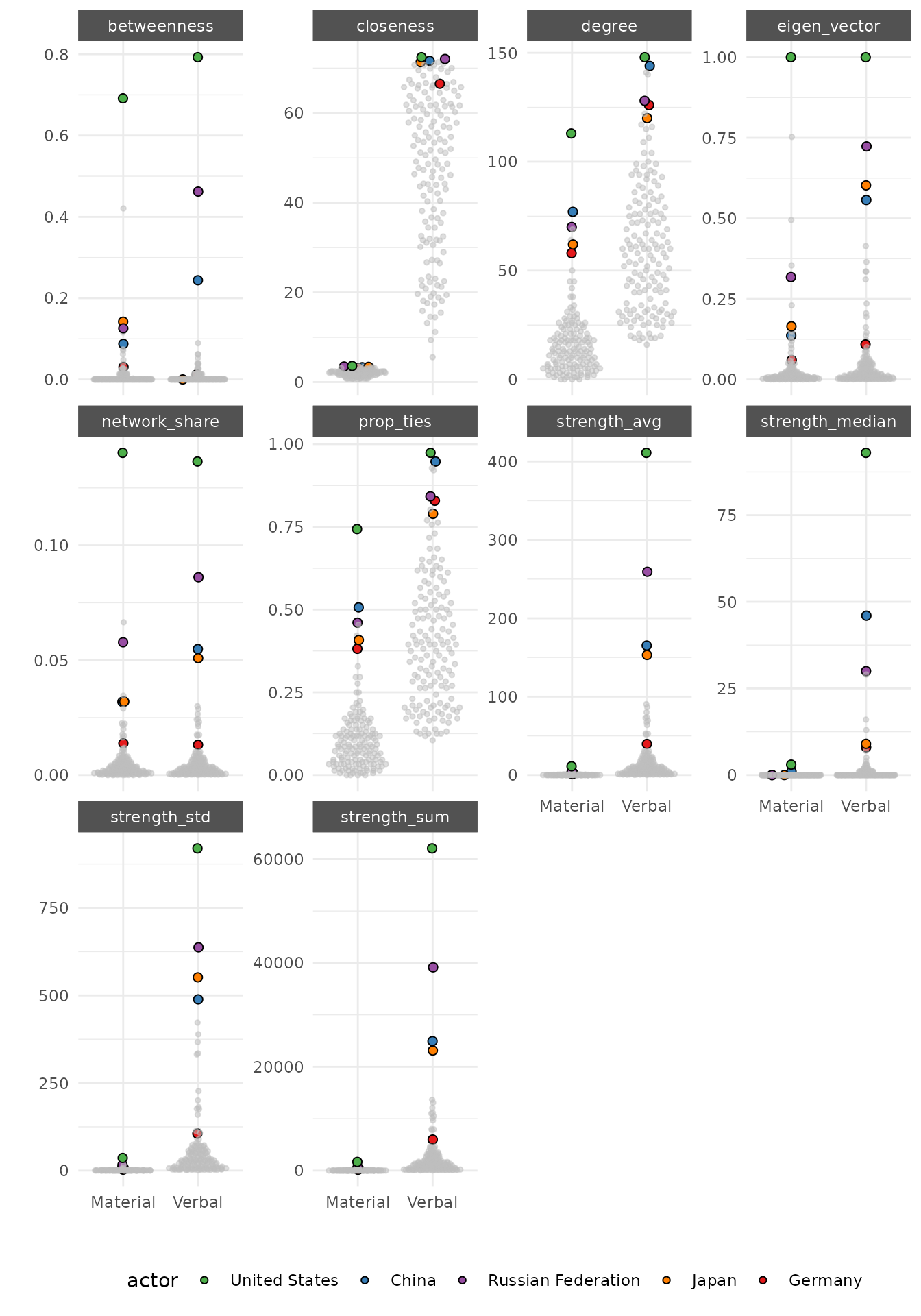
Power Analysis:

The US dominates both layers, confirming hegemonic status
Russia shows high verbal but lower material engagement – influence through diplomacy rather than resources
China (in 2002) shows moderate engagement, presaging its later rise
Japan’s material cooperation exceeds its diplomatic footprint
Germany balances both dimensions, reflecting EU leadership

Understanding Multiplexity: The Architecture of International Relations

Multiplexity analysis reveals which relationships involve multiple types of interaction – a key indicator of relationship depth and stability:

# Analyze edge patterns
verbal_melt <- melt(verbal_coop_net, remove_zeros = FALSE, na.rm = TRUE)
material_melt <- melt(material_coop_net, remove_zeros = FALSE, na.rm = TRUE)

edge_comparison <- merge(
    verbal_melt,
    material_melt,
    by = c("Var1", "Var2"),
    suffixes = c("_verbal", "_material")
) |>
    filter(value_verbal > 0 | value_material > 0)

# Categorize relationships
multiplexity_summary <- edge_comparison |>
    mutate(
        relationship_type = case_when(
            value_verbal > 0 & value_material > 0 ~ "Multiplex",
            value_verbal > 0 ~ "Verbal Only",
            value_material > 0 ~ "Material Only"
        )
    )

# Summary and visualization
table(multiplexity_summary$relationship_type)
#> 
#> Material Only     Multiplex   Verbal Only 
#>           124          2452          6926

ggplot(multiplexity_summary, aes(x = relationship_type)) +
    geom_bar() +
    labs(
        title = "The Multiplexity Gap in International Cooperation",
        subtitle = "Most relationships remain purely verbal",
        x = "Relationship Type",
        y = "Number of Country Pairs"
    ) +
    theme_minimal()

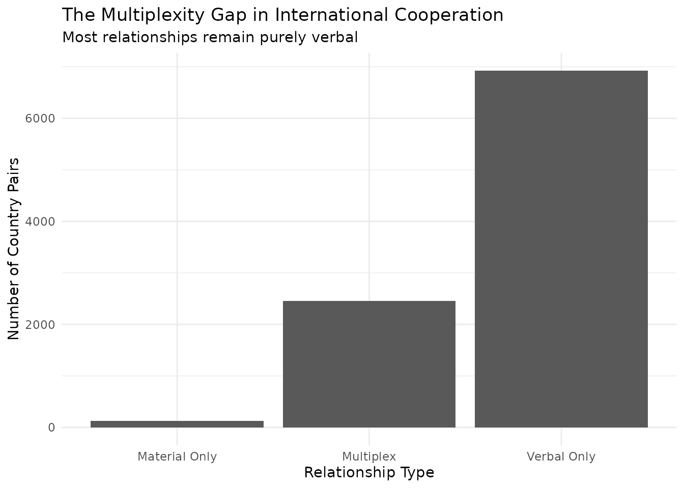
Multiplexity Insights:

Only 26% of relationships are multiplex (involving both verbal and material cooperation)
124 “material only” relationships deserve attention – these might represent covert cooperation or technical assistance below the diplomatic radar
The 2,452 multiplex relationships form the stable core of international cooperation

Who Has Multiplex Relationships?

# Identify multiplex relationships
multiplex_pairs <- multiplexity_summary |>
    filter(relationship_type == "Multiplex") |>
    mutate(total_coop = value_verbal + value_material) |>
    arrange(desc(total_coop)) |>
    head(10)

print("Strongest multiplex relationships:")
#> [1] "Strongest multiplex relationships:"
print(multiplex_pairs[, c("Var1", "Var2", "value_verbal", "value_material")])
#>                  Var1               Var2 value_verbal value_material
#> 1  Russian Federation      United States         5760             64
#> 2       United States Russian Federation         5760             64
#> 3              Israel      United States         4652             50
#> 4       United States             Israel         4652             50
#> 5               China      United States         4481             16
#> 6       United States              China         4481             16
#> 7               Japan      United States         4334             31
#> 8       United States              Japan         4334             31
#> 9            Pakistan      United States         3252            121
#> 10      United States           Pakistan         3252            121

US-Russia tops the list despite tensions, showing how former adversaries maintain multiple channels. US relationships with allies (Israel, Japan) and strategic competitors (China) also show high multiplexity, indicating relationship importance transcends simple friend/foe categories.

Advanced Analysis: Layer Dependencies

How Do Layers Relate?

# Comprehensive layer comparison
layer_comparison <- compare_networks(multilayer_net, what = "edges", method = "all")
print(layer_comparison)
#>           comparison correlation   jaccard  hamming qap_correlation qap_pvalue
#> 1 Verbal vs Material   0.4718002 0.2580509 0.305142       0.4718002          0
#>   spectral
#> 1 91163.55
#>             Verbal  Material
#> Verbal   1.0000000 0.4718002
#> Material 0.4718002 1.0000000
#>          Verbal Material
#> Verbal        0        0
#> Material      0        0
#> attr(,"n_perm")
#> [1] 5000

Key Metrics Explained:

Correlation (0.472): Moderate positive relationship – verbal cooperation somewhat predicts material cooperation
Jaccard (0.258): Only 26% edge overlap – most relationships exist in just one layer
Hamming (0.305): About 30% of possible edges differ between layers
QAP test (p < 0.001): The correlation is statistically significant, not due to chance

Visualizing Layer Relationships

# Cross-layer scatter
ggplot(edge_comparison, aes(x = log1p(value_verbal), y = log1p(value_material))) +
    geom_point(alpha = 0.2, color = "darkblue") +
    geom_smooth(method = "lm", color = "red", se = TRUE) +
    geom_density_2d(color = "gray", alpha = 0.5) +
    labs(
        title = "The Verbal-Material Cooperation Gap",
        subtitle = "Most relationships cluster along axes, not diagonal",
        x = "Log(Verbal Cooperation + 1)",
        y = "Log(Material Cooperation + 1)"
    ) +
    theme_minimal() +
    annotate("text", x = 7, y = 1, label = "Talk without action", fontface = "italic") +
    annotate("text", x = 1, y = 5, label = "Quiet support", fontface = "italic") +
    annotate("text", x = 6, y = 5, label = "Full cooperation", fontface = "italic")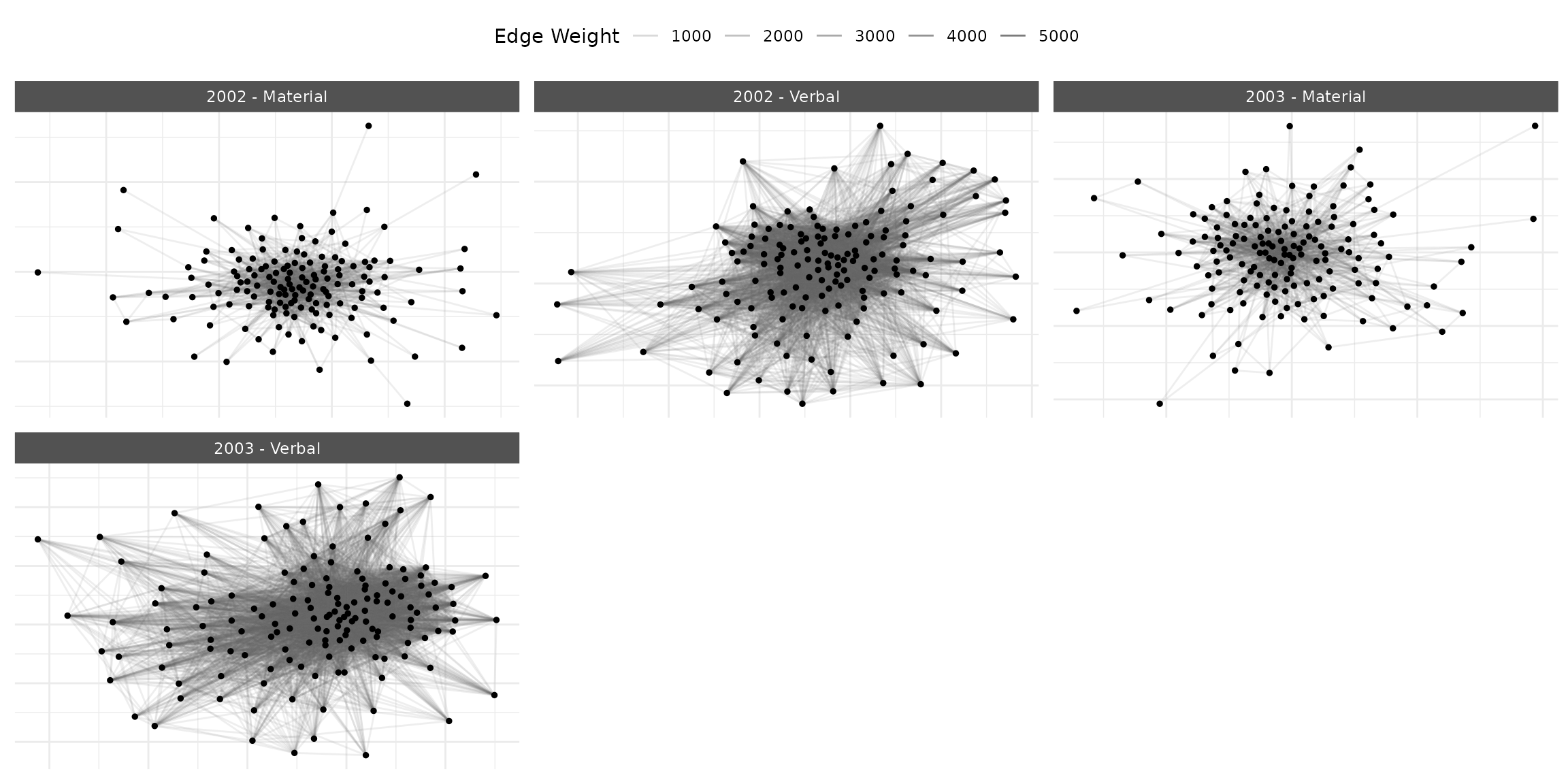

Temporal Dynamics in Multilayer Networks

Understanding how different layers evolve over time reveals changing cooperation dynamics:

# Create temporal multilayer network
years_example <- c(2001, 2002, 2003) # Around 9/11
icews_subset <- icews[icews$year %in% years_example, ]

verbal_temporal <- netify(
    icews_subset,
    actor1 = "i", actor2 = "j",
    time = "year",
    symmetric = TRUE,
    weight = "verbCoop"
)

material_temporal <- netify(
    icews_subset,
    actor1 = "i", actor2 = "j",
    time = "year",
    symmetric = TRUE,
    weight = "matlCoop"
)

temporal_multilayer <- layer_netify(
    list(verbal_temporal, material_temporal),
    layer_labels = c("Verbal", "Material")
)

# Visualize evolution
plot(temporal_multilayer,
    add_text = FALSE,
    facet_type = "wrap",
    facet_ncol = 3
)

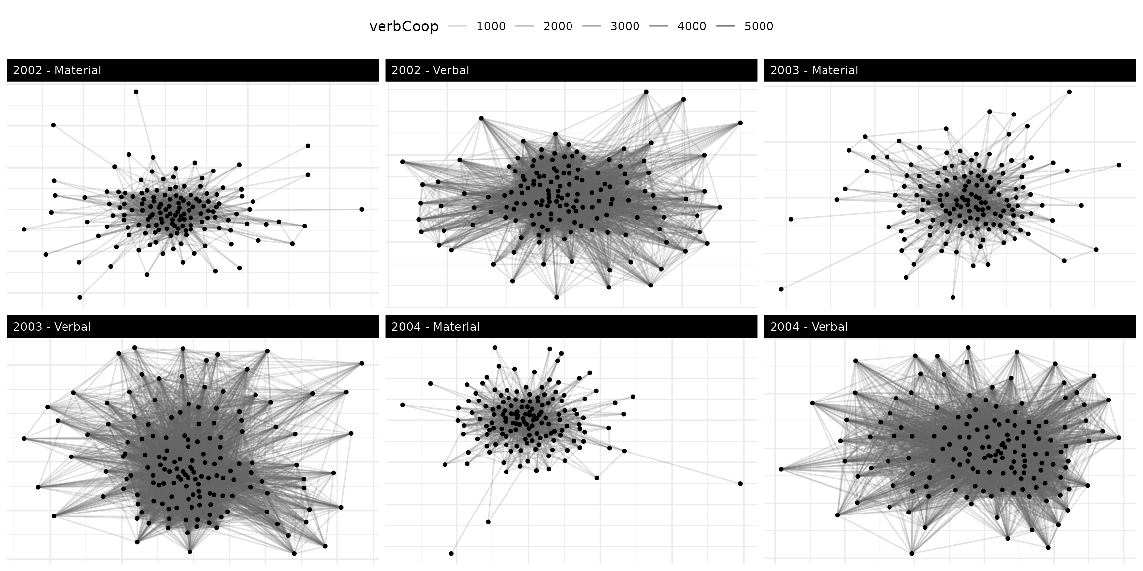
The post-9/11 period shows network evolution. Both layers densify from 2001 to 2003, but material cooperation grows more selectively, suggesting crisis-driven coalition building.

Practical Recommendations

When to Use Multilayer vs. Separate Analysis

Use multilayer when:

Relationships theoretically influence each other
You suspect substitution or complementarity effects
Actor positions might differ across relationship types
You need to identify relationship depth through multiplexity

Use separate analysis when:

Relationships are theoretically independent
Different actor sets across layers
Computational constraints exist
Initial exploration before multilayer modeling

Choosing Analysis Methods

For regime type effects: Use homophily() with “correlation” method for continuous variables like polity scores
For regional/categorical patterns: Use mixing_matrix() to see full interaction patterns
For relationship strength: Use compare_networks() with what="edges" and method="all" for comprehensive comparison
For individual actors: Use summary_actor() and examine layer-specific centralities

tl;dr

Multilayer network analysis in netify reveals how different types of political relationships interact, overlap, and diverge. By moving beyond single-layer analysis, we can:

Test more nuanced theories about international behavior
Identify actors with specialized roles across different domains
Understand the architecture of complex political systems
Track how relationship portfolios evolve over time
Most importantly … have fun!

Cassy Dorff and Shahryar Minhas

2025-06-30

Quick Start Example

Building Multilayer Networks: A Substantive Example

Visualizing Multilayer Structures

Basic Visualization with Interpretation

Comparing Network Structures

Testing Political Science Theories with Multilayer Networks

Theory 1: Democratic Peace in Different Domains

Theory 2: Regional Security Complexes

Theory 3: Conflict-Cooperation Dynamics

Identifying Strategic Actors

Who Bridges the Cooperation Gap?

Power Dynamics Across Layers

Understanding Multiplexity: The Architecture of International Relations

Who Has Multiplex Relationships?

Advanced Analysis: Layer Dependencies

How Do Layers Relate?

Visualizing Layer Relationships

Temporal Dynamics in Multilayer Networks

Practical Recommendations

When to Use Multilayer vs. Separate Analysis

Choosing Analysis Methods

tl;dr

Multilayer Networks

Cassy Dorff and Shahryar Minhas

2025-06-30

Why Multilayer Networks Matter for Social Science

Quick Start Example

Building Multilayer Networks: A Substantive Example

Visualizing Multilayer Structures

Basic Visualization with Interpretation

Comparing Network Structures

Testing Political Science Theories with Multilayer Networks

Theory 1: Democratic Peace in Different Domains

Theory 2: Regional Security Complexes

Theory 3: Conflict-Cooperation Dynamics

Identifying Strategic Actors

Who Bridges the Cooperation Gap?

Power Dynamics Across Layers

Understanding Multiplexity: The Architecture of International Relations

Who Has Multiplex Relationships?

Advanced Analysis: Layer Dependencies

How Do Layers Relate?

Visualizing Layer Relationships

Temporal Dynamics in Multilayer Networks

Practical Recommendations

When to Use Multilayer vs. Separate Analysis

Choosing Analysis Methods

tl;dr

references

Dorff, C., Gallop, M., & Minhas, S. (2020). Networks of Violence: Predicting Conflict in Nigeria. The Journal of Politics, 82(2), 476–493. https://doi.org/10.1086/706459
Minhas, S., Dorff, C., Gallop, M., Foster, M., Liu, H., Tellez, J., & Ward, M. D. (2022). Taking dyads seriously. Political Science Research and Methods, 10(4), 703–721. https://doi.org/10.1017/psrm.2021.56
Minhas, S., Hoff, P. D., & Ward, M. D. (2016). A new approach to analyzing coevolving longitudinal networks in international relations. Journal of Peace Research, 53(3), 491-505. https://doi.org/10.1177/0022343316630783