Foundations

Cassy Dorff and Shahryar Minhas

2026-06-05

package overview

You supply dyadic data, and netify turns it into network objects that work with summary, plotting, and modeling tools. The package is built for social-science network data, especially peace science data, but the same workflow works for many dyadic data sets.

This vignette walks through the main workflow: create a network, inspect it, plot it, add attributes, and pass it to other network packages.

The main workflow has three parts:

1. Create: Build network objects from dyadic data and attach nodal or dyadic variables.
2. Explore: Summarize networks at the graph and actor levels, then visualize the results.
3. Model: Prepare the network for other R network packages.

The table below lists common functions for each part of the workflow.

Create	Explore	Model
netify()	peek()	netify_to_amen()
add_node_vars()	summary_actor()	netify_to_igraph()
add_dyad_vars()	summary()	netify_to_statnet()
subset_netify()	plot_actor_stats()
	plot_graph_stats()
	plot()

netify begins with the user’s data input. Our core function, netify(), handles several different data inputs including data frames and edgelists (see documentation for more detail).

• The package can also create different types of networks including:

  • cross sectional networks
  • longitudinal (with static and varying actor composition)
  • bipartite networks
  • multilayer

• As well as create networks with different edge types:

  • weighted
  • binary
  • symmetric or non-symmetric

step 1: create

Begin by loading packages and supplying the data. We will use the peacesciencer package to grab some familiar data.

# load packages
library(netify)
library(peacesciencer)
library(dplyr)
library(ggplot2)

# organize external data for peacesciencer
peacesciencer::download_extdata()

# build a dyadic panel with peacesciencer
cow_dyads <- create_dyadyears(
    subset_years = c(1995:2014)
) |>
    # add mid data
    add_cow_mids() |>
    # add capital distance
    add_capital_distance() |>
    # add democracy
    add_democracy() |>
    # add gdp
    add_sim_gdp_pop(keep = c("pwtrgdp", "pwtpop"))

Next, create a netlet object from the COW data frame with netify(). The main arguments are:

• input is, in this use case, a dyadic data.frame that should have at the following variables used to specify actors:

  • actor1: names the first actor column
  • actor2: names the second actor column

• time names the period variable for longitudinal data.

• output_format sets the storage shape when you need one explicitly ("cross_sec", "longit_array", or "longit_list"); otherwise netify() picks from the input structure.

mid_long_network <- netify(
    input = cow_dyads,
    actor1 = "ccode1", actor2 = "ccode2", time = "year",
    weight = "cowmidonset",
    actor_time_uniform = FALSE,
    sum_dyads = FALSE, symmetric = TRUE,
    diag_to_NA = TRUE, missing_to_zero = TRUE,
    nodal_vars = c("v2x_polyarchy1", "v2x_polyarchy2"),
    dyad_vars = c("capdist"),
    dyad_vars_symmetric = c(TRUE)
)

## ! Converting `actor1` and/or `actor2` to character vector(s).

## ℹ `netify()` collapsed repeated actor-time rows before attaching nodal
##   variables.
## • Numeric nodal variables were averaged; non-numeric variables use the most
##   common non-missing value within each key.
## This message is displayed once per session.

You have created a network object.

You can also add nodal and dyadic data after creating the network with add_node_vars() and add_dyad_vars().

For example, add logged GDP for each actor-year:

# build one actor-year row for each node
node_data <- bind_rows(
    cow_dyads |>
        select(actor = ccode1, year, pwtrgdp = pwtrgdp1),
    cow_dyads |>
        select(actor = ccode2, year, pwtrgdp = pwtrgdp2)
) |>
    distinct(actor, year, .keep_all = TRUE) |>
    mutate(pwtrgdp_log = log(pwtrgdp + 1))

# attach the nodal variable
mid_long_network <- add_node_vars(
    netlet = mid_long_network,
    node_data = node_data,
    actor = "actor",
    time = "year"
)

# build a dyadic distance variable
cow_dyads$log_capdist <- log(cow_dyads$capdist + 1)

# attach the dyadic variable
mid_long_network <- add_dyad_vars(
    netlet = mid_long_network,
    dyad_data = cow_dyads,
    actor1 = "ccode1",
    actor2 = "ccode2",
    time = "year",
    dyad_vars = "log_capdist",
    dyad_vars_symmetric = TRUE
)

step 2: explore and summarize

We made a network, so let’s look at it. First, we might want to take a peek at the network object to see if the matrix looks the way we’d expect it to look. This function lets you glance at a specific slice of the network if it is longitudinal or the entire network if it is cross-sectional. (To actually subset the netlet object and make a new object use netify’s subset function.)

peek(mid_long_network,
    from = 5, to = 5,
    time = c("2009", "2010")
)

## $`2009`
##     100 101 110 115 130
## 100  NA   1   0   0   1
## 101   1  NA   0   0   0
## 110   0   0  NA   0   0
## 115   0   0   0  NA   0
## 130   1   0   0   0  NA
## 
## $`2010`
##     100 101 110 115 130
## 100  NA   1   0   0   0
## 101   1  NA   0   0   0
## 110   0   0  NA   0   0
## 115   0   0   0  NA   0
## 130   0   0   0   0  NA

Next, let’s examine a few basic summary statistics about the network using oursummary() function.

# build network-level summary statistics
mid_long_summary <- summary(mid_long_network)

We can also make a quick visualization of network statistics over time using the summary statistics data frame.

plot_graph_stats(mid_long_summary)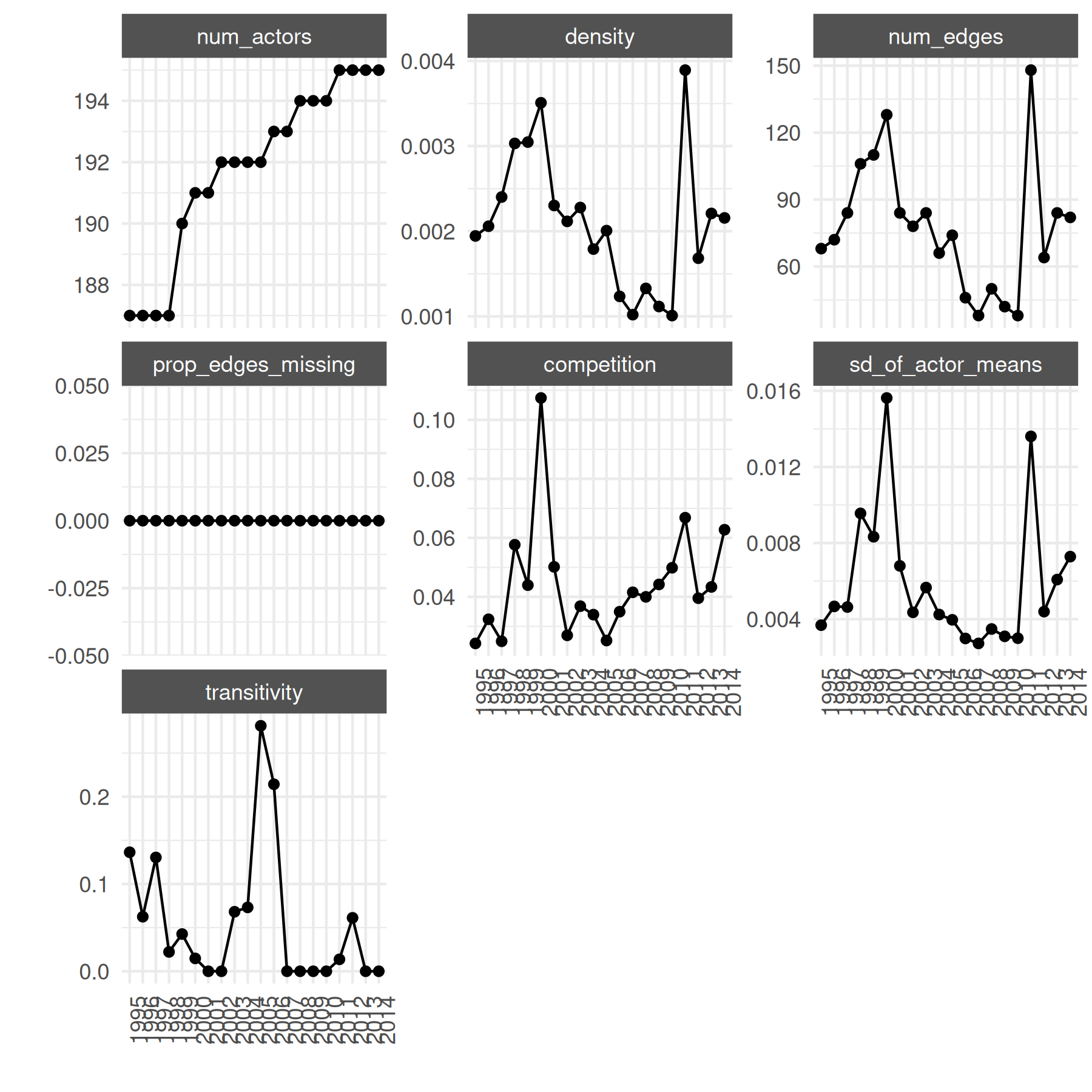

These graph statistics are useful for understanding changes over time at the network level. We might also want to look at actor-level statistics over time. The built-in summary_actor() function calculates actor-level degree, strength, and centrality statistics for each actor in each time period. The plot_actor_stats() function can show distributions across actors or trajectories for selected actors:

# summarize every actor-year
summary_actor_mids <- summary_actor(mid_long_network)
head(summary_actor_mids)

##   actor time degree   prop_ties network_share closeness betweenness
## 1   100 1995      1 0.005376344    0.01470588         1           0
## 2   101 1995      1 0.005376344    0.01470588         1           0
## 3   110 1995      0 0.000000000    0.00000000       NaN           0
## 4   115 1995      0 0.000000000    0.00000000       NaN           0
## 5   130 1995      1 0.005376344    0.01470588         1           0
## 6   135 1995      1 0.005376344    0.01470588         1           0
##   eigen_vector
## 1            0
## 2            0
## 3            0
## 4            0
## 5            0
## 6            0

We can look at the distribution of the statistic for all actors over time:

# plot actor-level distributions
plot_actor_stats(
    summary_actor_mids,
    across_actor = TRUE
)

## Warning: Removed 2913 rows containing non-finite outside the scale range
## (`stat_density_ridges()`).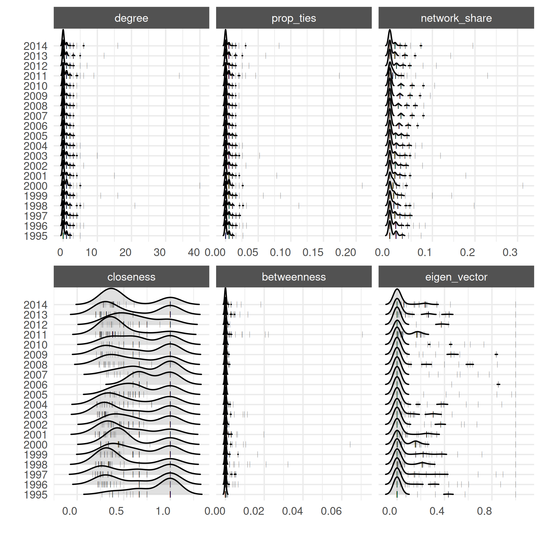

Or we might like to select a specific statistic to focus on across actors over time:

# focus on closeness
plot_actor_stats(
    summary_actor_mids,
    across_actor = TRUE,
    specific_stats = "closeness"
)

## Picking joint bandwidth of 0.114

## Warning: Removed 2913 rows containing non-finite outside the scale range
## (`stat_density_ridges()`).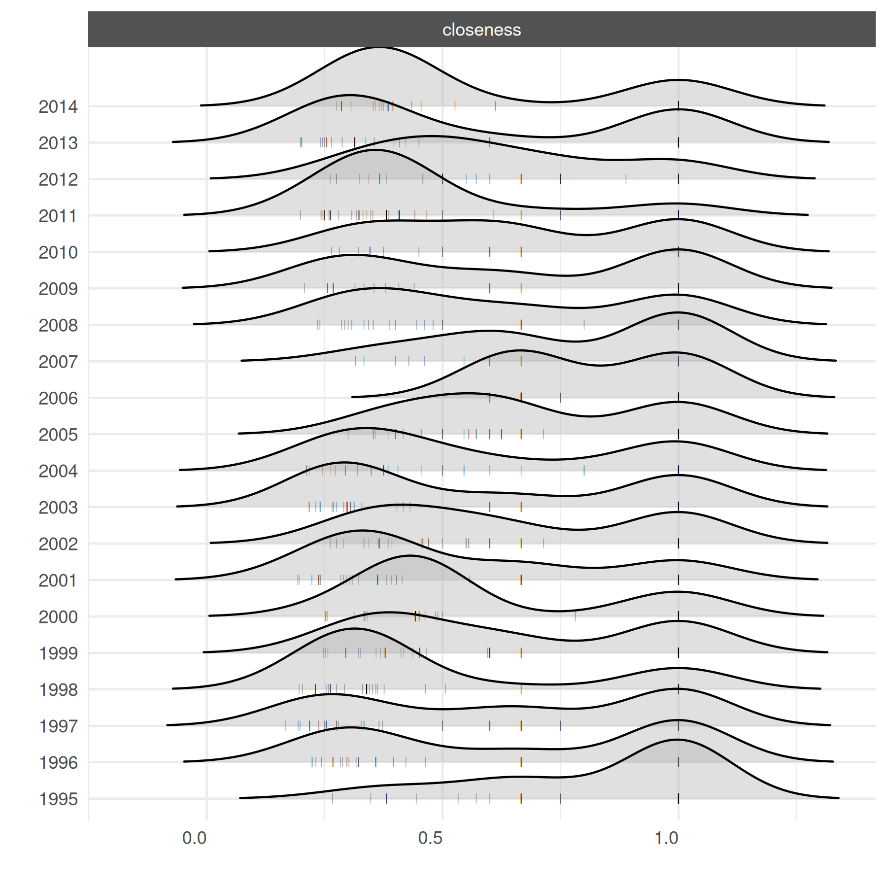

For actor-specific statistics over time, subset to a few actors so the plot stays legible.

# selected high-gdp countries
top_5 <- c("2", "710", "740", "255", "750")

plot_actor_stats(
    summary_actor_mids,
    across_actor = FALSE,
    specific_actors = top_5
)

## Warning: Removed 2058 rows containing missing values or values outside the scale range
## (`geom_line()`).

## Warning: Removed 2913 rows containing missing values or values outside the scale range
## (`geom_point()`).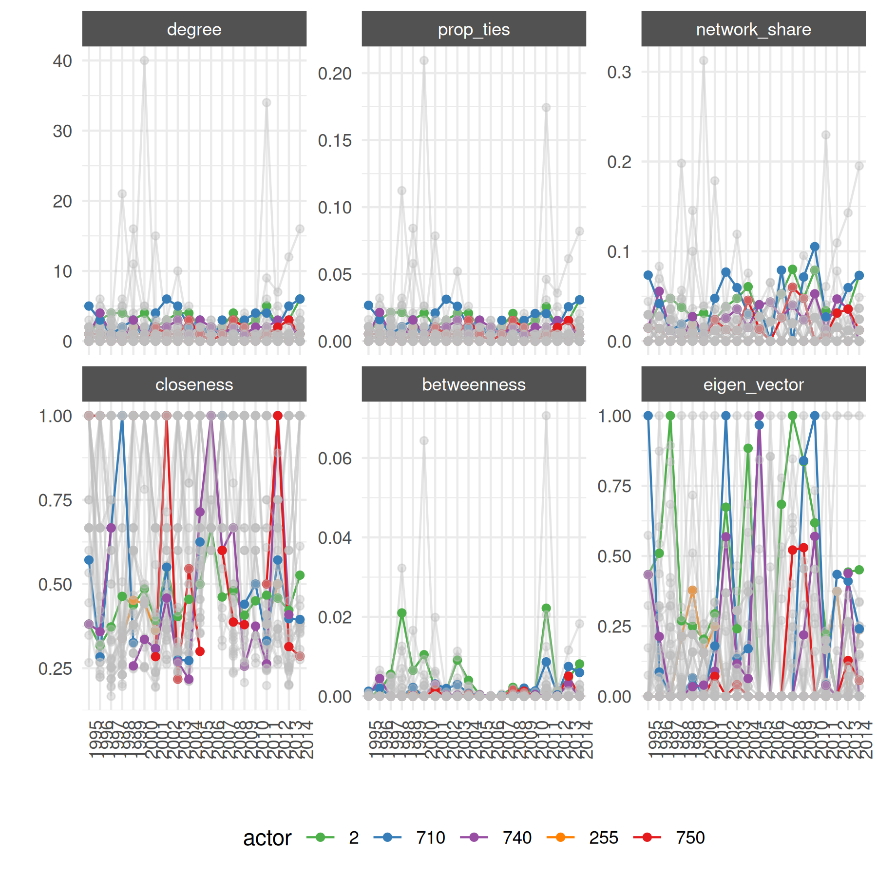

We can also zoom into a specific time slice of the network:

summary_df_static <- summary_actor_mids[summary_actor_mids$time == 2011, ]

plot_actor_stats(
    summary_df_static,
    across_actor = FALSE,
    specific_actors = top_5
)

## ! Note: The `summary_df` provided only has one unique time point, so longitudinal will be set to FALSE.

## Warning: Removed 123 rows containing missing values or values outside the scale range
## (`position_quasirandom()`).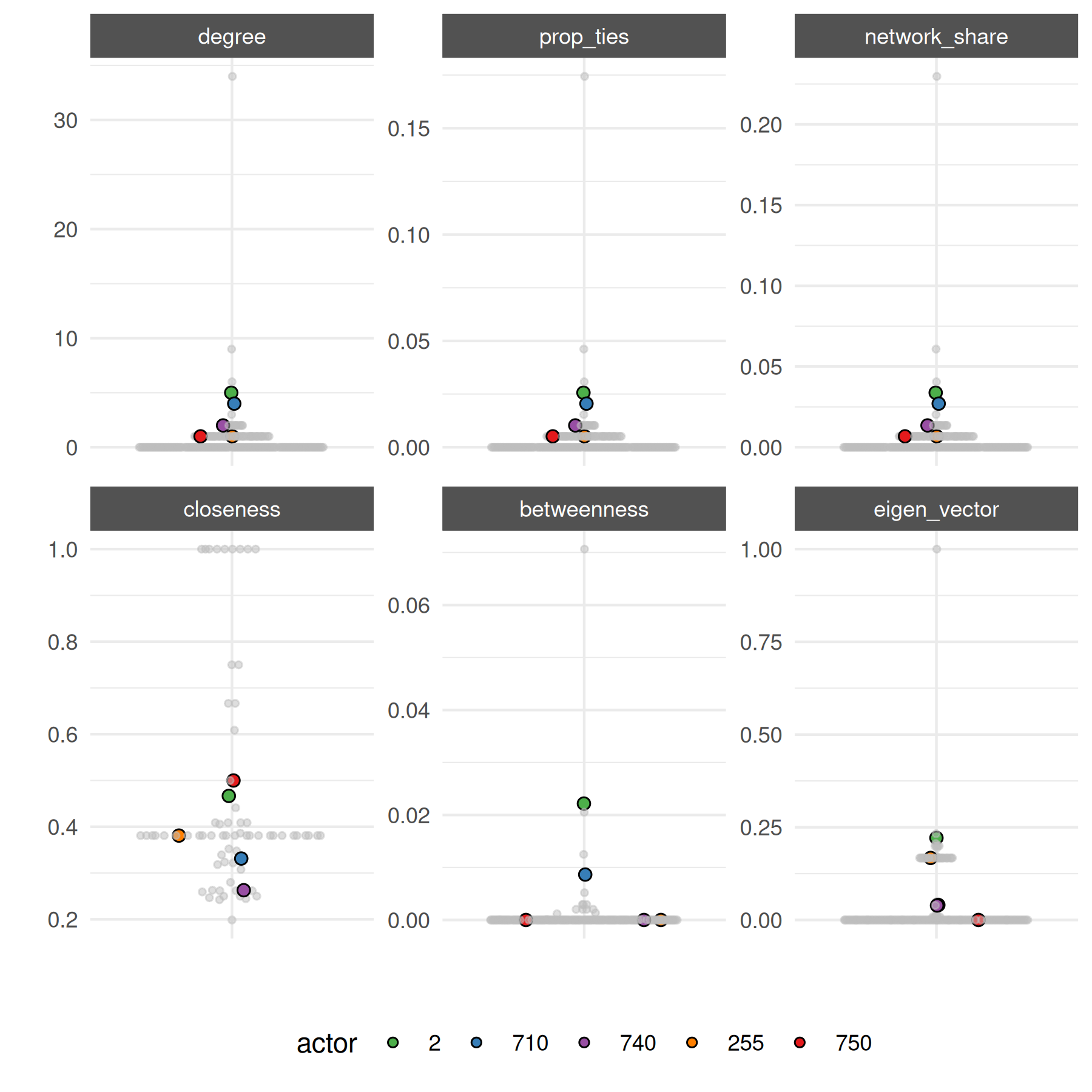

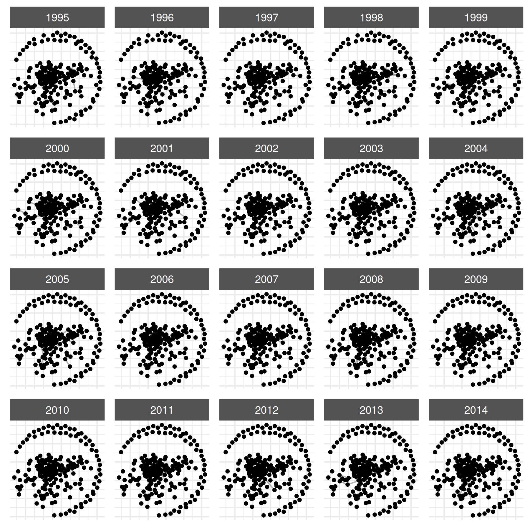
Instead of looking at summary statistics, we also might want to simply visualize the entire network. We can do this by plotting the netify object.

By default, plot() uses auto_format = TRUE, which automatically adjusts aesthetics based on your network’s properties — node sizes scale down for larger networks, edge transparency increases for denser networks, and text labels appear for small networks (≤15 nodes). You can disable this with auto_format = FALSE for full manual control, or simply override any individual parameter.

# default plot with auto_format
plot(mid_long_network,
    static_actor_positions = TRUE,
    remove_isolates = FALSE
)

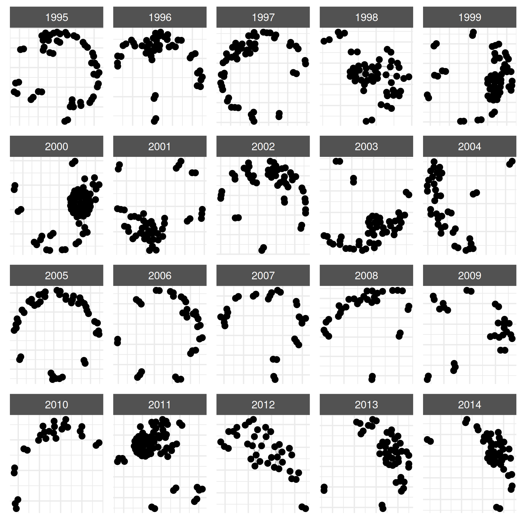
# override specific defaults
plot(
    mid_long_network,
    edge_color = "grey",
    node_size = 2
)

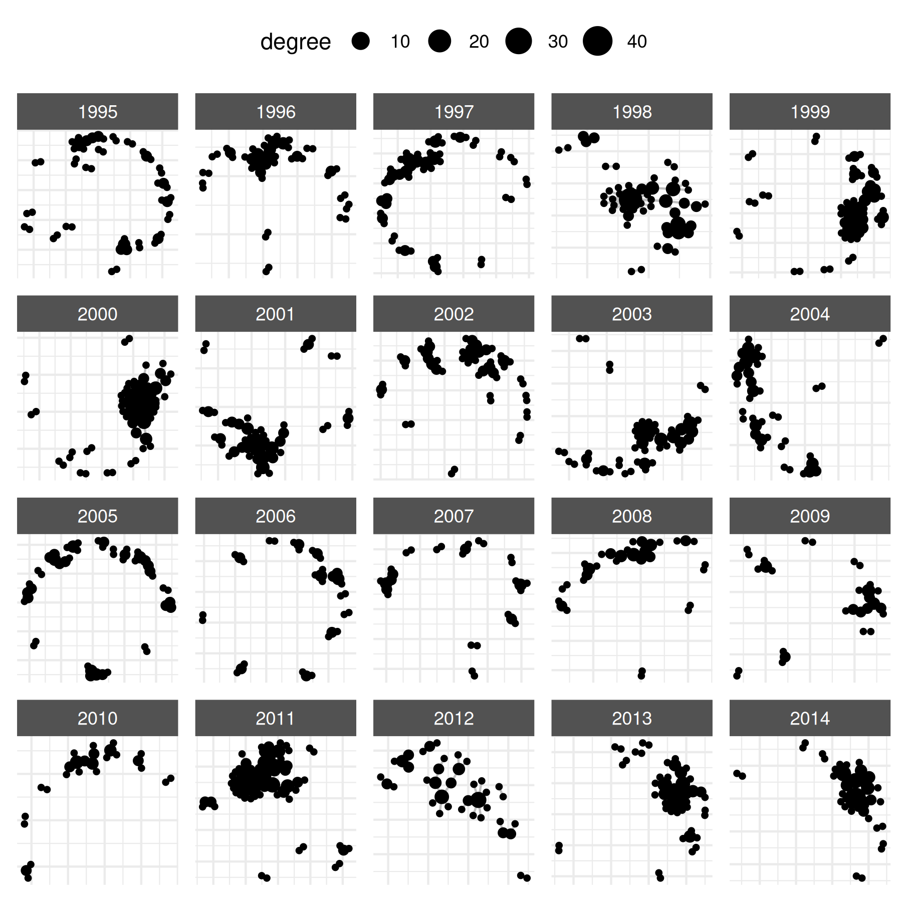
You can also map actor-level summary statistics onto the network plot.

# attach actor statistics
mid_long_network <- add_node_vars(
    mid_long_network,
    summary_actor_mids,
    actor = "actor", time = "time",
    node_vars = c("degree", "prop_ties", "eigen_vector"),
)

Print the object to inspect its metadata.

# inspect the netlet object
print(mid_long_network)

## ✔ Network data created.
## • Unipartite
## • Symmetric
## • Weights from `cowmidonset`
## • Longitudinal: 20 Periods
## • # Unique Actors: 195
## Network Summary Statistics (averaged across time):
##              dens miss trans
## cowmidonset 0.002    0 0.056
## • Nodal Features: v2x_polyarchy1, v2x_polyarchy2, pwtrgdp, pwtrgdp_log, degree,
## prop_ties, eigen_vector
## • Dyad Features: capdist, log_capdist

The nodal attributes are stored on the object.

# inspect nodal data
head(
    attr(
        mid_long_network,
        "nodal_data"
    )
)

##   actor time v2x_polyarchy1 v2x_polyarchy2  pwtrgdp pwtrgdp_log degree
## 1     2 1995          0.868      0.4767047 13375583    16.40894      1
## 2     2 1996          0.867      0.4741600 14136908    16.46430      3
## 3     2 1997          0.866      0.4898562 14480122    16.48829      4
## 4     2 1998          0.867      0.4879351 15268303    16.54129      4
## 5     2 1999          0.870      0.4921494 16085312    16.59342      3
## 6     2 2000          0.868      0.4940449 16191328    16.59999      4
##     prop_ties eigen_vector
## 1 0.005376344    0.4334163
## 2 0.016129032    0.5097062
## 3 0.021505376    1.0000000
## 4 0.021505376    0.2690264
## 5 0.015873016    0.2492445
## 6 0.021052632    0.2037526

head(attributes(mid_long_network)$nodal_data)

##   actor time v2x_polyarchy1 v2x_polyarchy2  pwtrgdp pwtrgdp_log degree
## 1     2 1995          0.868      0.4767047 13375583    16.40894      1
## 2     2 1996          0.867      0.4741600 14136908    16.46430      3
## 3     2 1997          0.866      0.4898562 14480122    16.48829      4
## 4     2 1998          0.867      0.4879351 15268303    16.54129      4
## 5     2 1999          0.870      0.4921494 16085312    16.59342      3
## 6     2 2000          0.868      0.4940449 16191328    16.59999      4
##     prop_ties eigen_vector
## 1 0.005376344    0.4334163
## 2 0.016129032    0.5097062
## 3 0.021505376    1.0000000
## 4 0.021505376    0.2690264
## 5 0.015873016    0.2492445
## 6 0.021052632    0.2037526

And now return to our network graph by highlighting specific nodal attributes. To map visual properties to data, we use the node_*_by naming convention (e.g., node_size_by, node_color_by). The legacy point_*_var names (e.g., point_size_var) also work identically if you prefer that style.

# vary node size by degree
plot(
    mid_long_network,
    edge_color = "grey",
    node_size_by = "degree"
)

# vary node color by polyarchy
plot(
    mid_long_network,
    edge_color = "grey",
    node_size_by = "degree",
    node_color_by = "v2x_polyarchy1",
    node_color_label = "Polyarchy",
    node_size_label = "Degree"
) +
    scale_color_gradient2()

## Scale for colour is already present.
## Adding another scale for colour, which will replace the existing scale.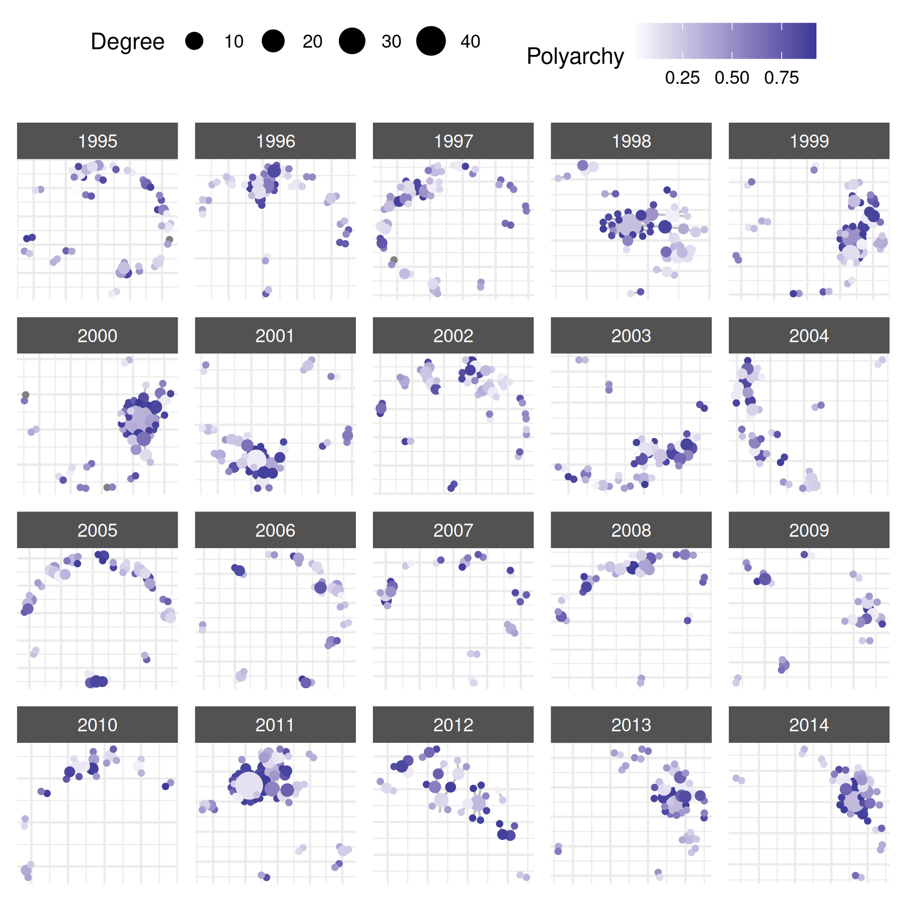

We might also prefer to add labels, but only a select few:

library(countrycode)
cowns <- countrycode(
    c(
        "United States", "China", "Russia",
        "France", "Germany", "United Kingdom"
    ),
    "country.name", "cown"
)
cabbs <- countrycode(cowns, "cown", "iso3c")

plot(
    mid_long_network,
    edge_color = "grey",
    node_size_by = "degree",
    node_color_by = "v2x_polyarchy1",
    node_color_label = "Polyarchy",
    node_size_label = "Degree",
    select_text = cowns,
    select_text_display = cabbs,
    text_size = 3
) +
    scale_color_gradient2()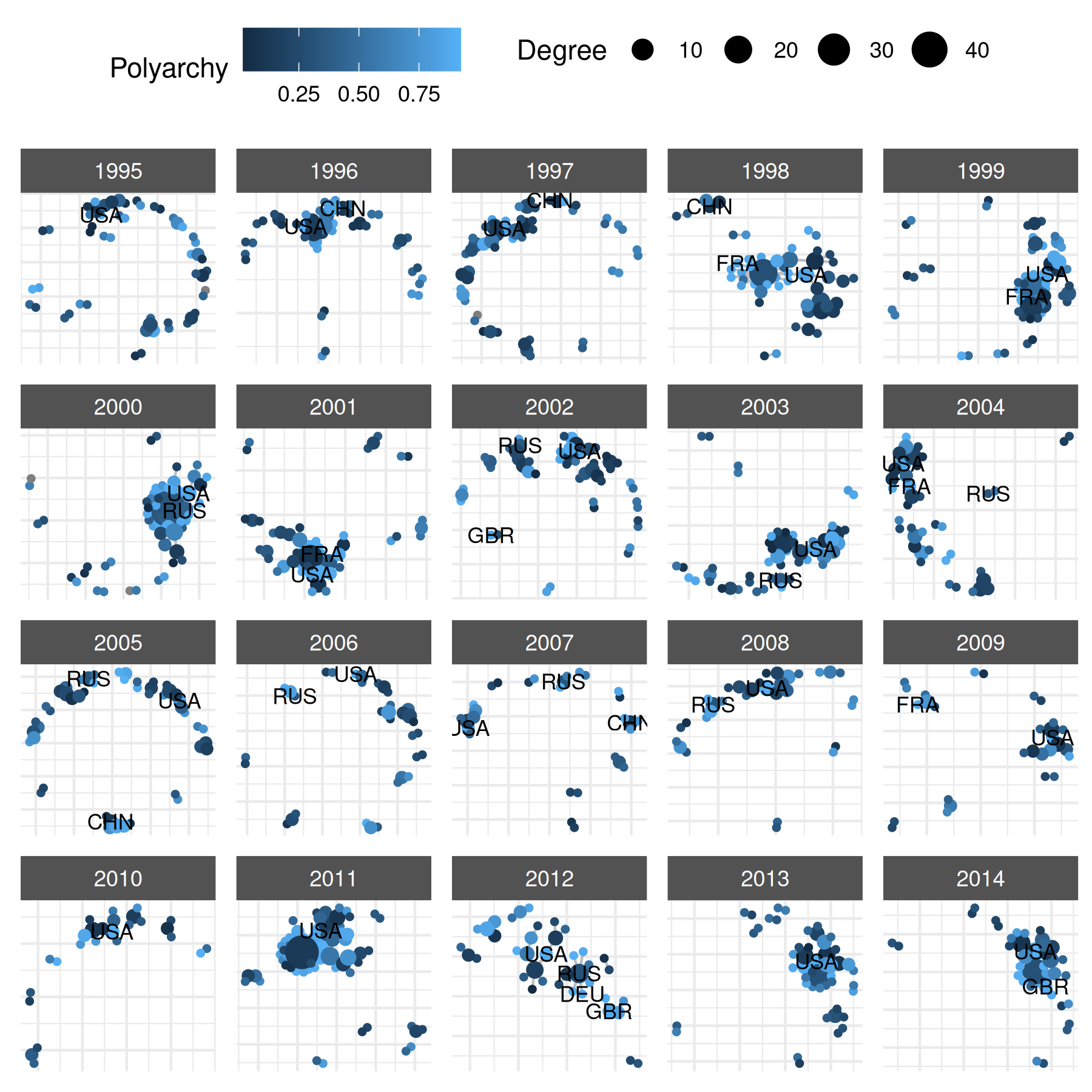

# draw labels without points
plot(
    mid_long_network,
    edge_color = "grey",
    add_points = FALSE,
    add_label = TRUE,
    label_size_var = "degree",
    label_color = "white",
    label_fill_var = "v2x_polyarchy1",
    label_fill_label = "Polyarchy",
    label_size_label = "Degree"
) + guides(size = "none")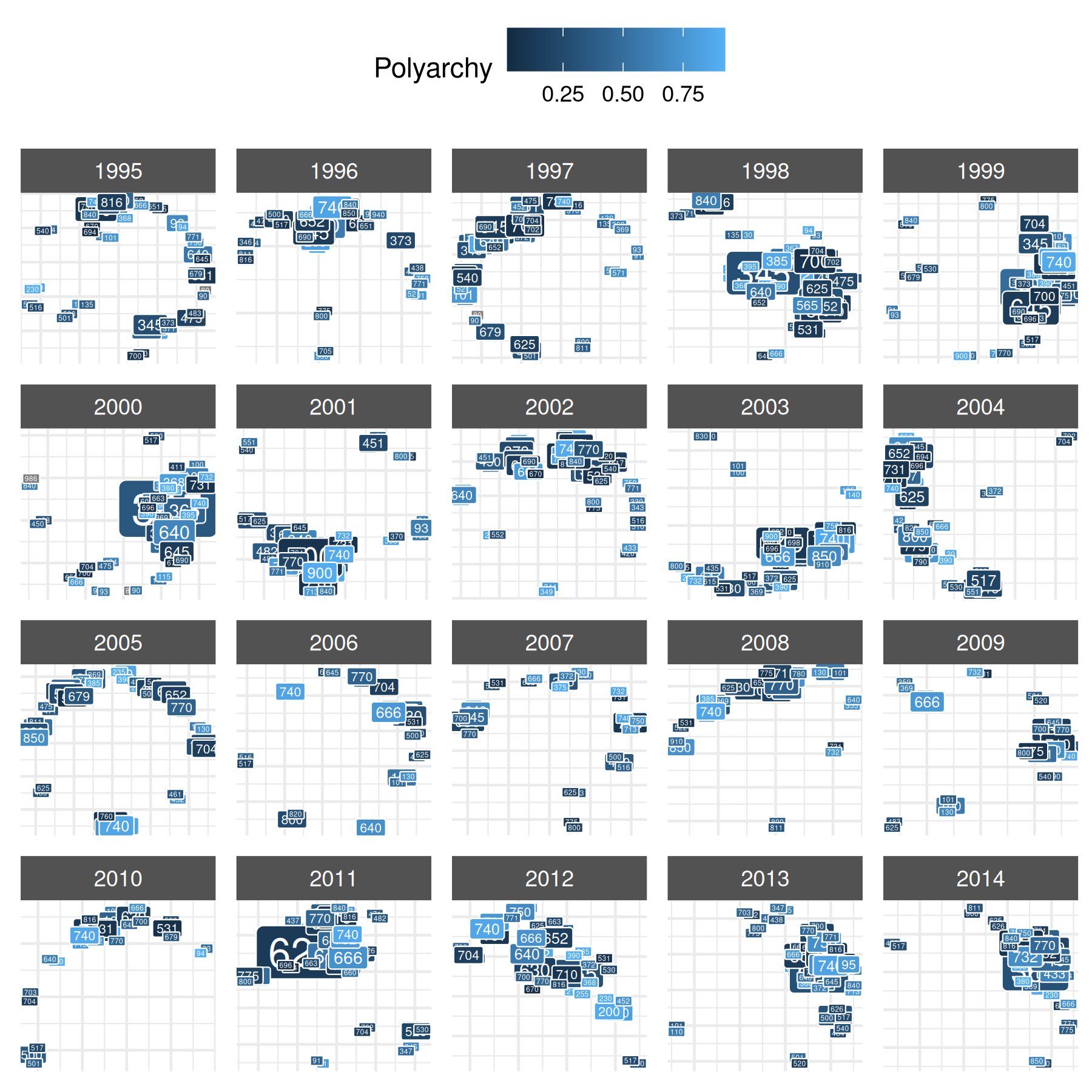

extracting data back to a data frame

If you need to convert a netify object back into a dyadic data frame — for example, to run regressions or export to other software — use unnetify():

mid_long_df <- unnetify(mid_long_network)
head(mid_long_df[, 1:5])

##   from  to time cowmidonset   capdist
## 1  100 101 1995           1 1024.5480
## 2  100 110 1995           0 1779.6330
## 3  100 115 1995           0 2101.0041
## 4  100 130 1995           0  732.7128
## 5  100 135 1995           0 1889.2499
## 6  100 140 1995           0 2853.6456

This returns one row per dyad with all nodal and dyadic attributes merged in. Use remove_zeros = TRUE to keep only non-zero edges for a more compact result.

step 3: model

After creating and exploring the network, you can pass it to other modeling packages. The examples below use a cross-sectional network.

First, prepare the data:

# prepare cross-sectional data
cow_cross <- cow_dyads |>
    group_by(ccode1, ccode2) |>
    summarize(
        cowmidonset = ifelse(any(cowmidonset > 0), 1, 0),
        capdist = mean(capdist),
        polity21 = mean(polity21, na.rm = TRUE),
        polity22 = mean(polity22, na.rm = TRUE),
        pwtrgdp1 = mean(pwtrgdp1, na.rm = TRUE),
        pwtrgdp2 = mean(pwtrgdp2, na.rm = TRUE),
        pwtpop1 = mean(pwtpop1, na.rm = TRUE),
        pwtpop2 = mean(pwtpop2, na.rm = TRUE)
    ) |>
    ungroup() |>
    mutate(
        capdist = log(capdist + 1)
    )

# subset to actors with average population above 10 million
actor_to_keep <- cow_cross |>
    select(ccode1, pwtpop1) |>
    filter(pwtpop1 > 10) |>
    distinct(ccode1)

# filter cow_cross by actor_to_keep
cow_cross <- cow_cross |>
    filter(ccode1 %in% actor_to_keep$ccode1) |>
    filter(ccode2 %in% actor_to_keep$ccode1)

# build cross-sectional netlet
mid_cross_network <- netify(
    cow_cross,
    actor1 = "ccode1", actor2 = "ccode2",
    weight = "cowmidonset",
    sum_dyads = FALSE, symmetric = TRUE,
    diag_to_NA = TRUE, missing_to_zero = FALSE,
    nodal_vars = c(
        "polity21", "polity22", "pwtrgdp1",
        "pwtrgdp2", "pwtpop1", "pwtpop2"
    ),
    dyad_vars = c("capdist"),
    dyad_vars_symmetric = c(TRUE)
)

Next, pass the netify object to amen. This section requires the amen package (install.packages("amen")).

library(amen)

# prepare amen inputs
mid_cross_amen <- netify_to_amen(mid_cross_network)

# inspect amen inputs
str(mid_cross_amen)

## List of 4
##  $ Y    : num [1:86, 1:86] NA 1 1 0 0 0 0 0 0 0 ...
##   ..- attr(*, "dimnames")=List of 2
##   .. ..$ : chr [1:86] "100" "101" "130" "135" ...
##   .. ..$ : chr [1:86] "100" "101" "130" "135" ...
##  $ Xdyad: num [1:86, 1:86, 1] 0 6.93 6.6 7.54 7.96 ...
##   ..- attr(*, "dimnames")=List of 3
##   .. ..$ : chr [1:86] "100" "101" "130" "135" ...
##   .. ..$ : chr [1:86] "100" "101" "130" "135" ...
##   .. ..$ : chr "capdist"
##  $ Xrow : num [1:86, 1:6] 7 4.3 6.38 6.28 8 ...
##   ..- attr(*, "dimnames")=List of 2
##   .. ..$ : chr [1:86] "100" "101" "130" "135" ...
##   .. ..$ : chr [1:6] "polity21" "polity22" "pwtrgdp1" "pwtrgdp2" ...
##  $ Xcol : num [1:86, 1:6] 7 4.3 6.38 6.28 8 ...
##   ..- attr(*, "dimnames")=List of 2
##   .. ..$ : chr [1:86] "100" "101" "130" "135" ...
##   .. ..$ : chr [1:6] "polity21" "polity22" "pwtrgdp1" "pwtrgdp2" ...

# fit amen model
mid_amen_mod <- ame(
    Y = mid_cross_amen$Y,
    Xdyad = mid_cross_amen$Xdyad,
    family = "bin",
    R = 0,
    symmetric = TRUE,
    seed = 6886,
    nscan = 50,
    burn = 10,
    odens = 1,
    plot = FALSE,
    print = FALSE
)

We can apply the same process to ERGMs. This section requires the ergm package (install.packages("ergm")).

library(ergm)

## Loading required package: network

## 
## 'network' 1.20.0 (2026-02-06), part of the Statnet Project
## * 'news(package="network")' for changes since last version
## * 'citation("network")' for citation information
## * 'https://statnet.org' for help, support, and other information

## Registered S3 methods overwritten by 'ergm':
##   method               from
##   simulate.formula     lme4
##   simulate.formula_lhs lme4

## 
## 'ergm' 4.12.0 (2026-02-17), part of the Statnet Project
## * 'news(package="ergm")' for changes since last version
## * 'citation("ergm")' for citation information
## * 'https://statnet.org' for help, support, and other information

## 'ergm' 4 is a major update that introduces some backwards-incompatible
## changes. Please type 'news(package="ergm")' for a list of major
## changes.

# netify_to_statnet converts to a network object,
# which is what ergm uses
mid_cross_ergm <- netify_to_statnet(mid_cross_network)

## ! Nodal columns with "NA" detected: "polity21". Ergm terms like
##   `nodecov()`/`nodematch()` will refuse to fit.
## ℹ Use `drop_na_actors(net, cols = c('polity21'))` (or impute) before refitting.
## This message is displayed once per session.

## ℹ Dyad covariates attached as per-edge attributes under "capdist_e" and as
##   network-level matrices under their original names ("capdist").
## ℹ For `ergm::edgecov()` use the matrix name (e.g. `edgecov('capdist')`); the
##   "_e" per-edge attribute is for descriptive use such as edge styling.
## This message is displayed once per session.

# inspect statnet attributes
mid_cross_ergm

##  Network attributes:
##   vertices = 86 
##   directed = FALSE 
##   hyper = FALSE 
##   loops = FALSE 
##   multiple = FALSE 
##   bipartite = FALSE 
##   cowmidonset: 86x86 matrix
##   capdist: 86x86 matrix
##   total edges= 149 
##     missing edges= 0 
##     non-missing edges= 149 
## 
##  Vertex attribute names: 
##     polity21 polity22 pwtpop1 pwtpop2 pwtrgdp1 pwtrgdp2 vertex.names 
## 
##  Edge attribute names: 
##     capdist_e cowmidonset

# replace missing nodecov values for the example
set.vertex.attribute(
    mid_cross_ergm, "polity21", 
    ifelse(
        is.na(get.vertex.attribute(mid_cross_ergm, "polity21")), 
        0, get.vertex.attribute(mid_cross_ergm, "polity21")))

set.vertex.attribute(
    mid_cross_ergm, "pwtrgdp2",
    ifelse(
        is.na(get.vertex.attribute(mid_cross_ergm, "pwtrgdp2")),
        0, get.vertex.attribute(mid_cross_ergm, "pwtrgdp2")) )

set.vertex.attribute(
    mid_cross_ergm, "pwtpop2",
    ifelse(
        is.na(get.vertex.attribute(mid_cross_ergm, "pwtpop2")),
        0,  get.vertex.attribute(mid_cross_ergm, "pwtpop2")) )

# fit ergm model
ergm_model <- ergm(
    formula = mid_cross_ergm ~
        edges +
        nodecov("polity21") +
        nodecov("pwtrgdp2") +
        nodecov("pwtpop2")
)

## Starting maximum pseudolikelihood estimation (MPLE):
## Obtaining the responsible dyads.
## Evaluating the predictor and response matrix.
## Maximizing the pseudolikelihood.
## Finished MPLE.
## Evaluating log-likelihood at the estimate.

references

• Csárdi G, Nepusz T, Traag V, Horvát S, Zanini F, Noom D, Müller K (2024). igraph: Network Analysis and Visualization in R. doi:10.5281/zenodo.7682609, R package version 2.0.3, https://CRAN.R-project.org/package=igraph.

• Davies, Shawn, Therese Pettersson & Magnus Öberg (2023). Organized violence 1989-2022 and the return of conflicts between states?. Journal of Peace Research 60(4).

• Handcock M, Hunter D, Butts C, Goodreau S, Krivitsky P, Morris M (2018). ergm: Fit, Simulate and Diagnose Exponential-Family Models for Networks. The Statnet Project (https://statnet.org/). R package version 3.9.4, https://CRAN.R-project.org/package=ergm.

• Hoff, Peter D. “Dyadic data analysis with amen.” arXiv preprint arXiv:1506.08237 (2015).

• Högbladh Stina, 2023, “UCDP GED Codebook version 23.1”, Department of Peace and Conflict Research, Uppsala University

• Miller S (2022). “peacesciencer: An R Package for Quantitative Peace Science Research.” Conflict Management and Peace Science, 39(6), 755–779. doi: 10.1177/07388942221077926.

• Statnet Development Team (Pavel N. Krivitsky, Mark S. Handcock, David R. Hunter, Carter T. Butts, Chad Klumb, Steven M. Goodreau, and Martina Morris) (2003-2023). statnet: Software tools for the Statistical Modeling of Network Data. URL https://statnet.org/

• Sundberg, Ralph and Erik Melander (2013) Introducing the UCDP Georeferenced Event Dataset. Journal of Peace Research 50(4).