Tracking Changes in Cooperation and Conflict: Comparing Networks

Vignette Summary

This vignette demonstrates how to use netify to analyze changes in international relations over time using data from the Integrated Crisis Early Warning System (ICEWS). We’ll explore some fun questions about how countries interact:

Talk vs. Action: Do countries that cooperate verbally (diplomatic statements) also cooperate materially (aid, trade)?
Friend or Foe: Are cooperation and conflict separate networks, or do countries that cooperate also tend to have conflicts?
Temporal Stability: Which international relationships persist over time and which are fleeting?
Structural Evolution: How do the overall patterns of international interactions change across years?

We’ll use compare_networks() to answer these questions:

compare_networks():

Compares networks across multiple dimensions - edges, structure, nodes, and attributes. Think of it as running a comprehensive diagnostic between any two (or more) networks to understand what’s similar, what’s different, and why it matters.
Function notes:
- Multi-method flexibility: Choose from correlation, Jaccard, Hamming, QAP, spectral distance, or “all”
- Four comparison modes: Compare edges (who connects to whom), structure (density, clustering), nodes (actor composition), or attributes (actor characteristics)
- Statistical rigor: Built-in permutation tests for significance
- Output: Returns information on edge changes, similarity metrics, and structural differences

library(netify)
library(ggplot2)
library(tidyverse)
library(patchwork)

Understanding ICEWS Data

The Integrated Crisis Early Warning System (ICEWS) provides event-level data on interactions between international actors. Each event captures:

Who: Source and target countries
What: Type of interaction (cooperation or conflict, verbal or material)
When: Date of the event
How Much: Intensity scores on cooperation/conflict scales

# Load ICEWS data
data(icews)

# Take a peek
head(icews)

##             i       j year                       id verbCoop matlCoop verbConf
## 2 Afghanistan Albania 2002 AFGHANISTAN_ALBANIA_2002        6        1        0
## 3 Afghanistan Albania 2003 AFGHANISTAN_ALBANIA_2003        1        1        0
## 4 Afghanistan Albania 2004 AFGHANISTAN_ALBANIA_2004       10        2        0
## 5 Afghanistan Albania 2005 AFGHANISTAN_ALBANIA_2005        0        0        0
## 6 Afghanistan Albania 2006 AFGHANISTAN_ALBANIA_2006        6        2        3
## 7 Afghanistan Albania 2007 AFGHANISTAN_ALBANIA_2007        3        2        0
##   matlConf           i_year       j_year i_polity2 j_polity2 i_iso3c j_iso3c
## 2        0 AFGHANISTAN_2002 ALBANIA_2002        NA         7     AFG     ALB
## 3        0 AFGHANISTAN_2003 ALBANIA_2003        NA         7     AFG     ALB
## 4        1 AFGHANISTAN_2004 ALBANIA_2004        NA         7     AFG     ALB
## 5        0 AFGHANISTAN_2005 ALBANIA_2005        NA         9     AFG     ALB
## 6       21 AFGHANISTAN_2006 ALBANIA_2006        NA         9     AFG     ALB
## 7        0 AFGHANISTAN_2007 ALBANIA_2007        NA         9     AFG     ALB
##     i_region              j_region       i_gdp      j_gdp i_log_gdp j_log_gdp
## 2 South Asia Europe & Central Asia  7555185296 6857137321  22.74550  22.64856
## 3 South Asia Europe & Central Asia  8222480251 7236243584  22.83014  22.70237
## 4 South Asia Europe & Central Asia  8338755823 7635298387  22.84418  22.75605
## 5 South Asia Europe & Central Asia  9275174321 8057257368  22.95061  22.80984
## 6 South Asia Europe & Central Asia  9772082812 8532849798  23.00280  22.86719
## 7 South Asia Europe & Central Asia 11123202208 9043392346  23.13230  22.92530
##      i_pop   j_pop i_log_pop j_log_pop
## 2 21000256 3051010  16.86005  14.93098
## 3 22645130 3039616  16.93546  14.92724
## 4 23553551 3026939  16.97479  14.92306
## 5 24411191 3011487  17.01055  14.91794
## 6 25442944 2992547  17.05195  14.91164
## 7 25903301 2970017  17.06988  14.90408

The quad variables in ICEWS:

verbCoop: Verbal cooperation (diplomatic statements, promises)
matlCoop: Material cooperation (aid, trade agreements)
verbConf: Verbal conflict (threats, accusations)
matlConf: Material conflict (sanctions, military actions)

Creating Networks for Comparison

First, let’s create separate networks for different types of interactions in a single year:

# Create networks for different interaction types in 2002
icews_2002 <- icews[icews$year == 2002, ]

# Verbal cooperation network
verb_coop_2002 <- netify(
    icews_2002,
    actor1 = "i", actor2 = "j",
    weight = "verbCoop",
    symmetric = FALSE,
    nodal_vars = c('i_polity2', 'i_log_gdp', 'i_region')
)

# Material cooperation network
matl_coop_2002 <- netify(
    icews_2002,
    actor1 = "i", actor2 = "j",
    weight = "matlCoop",
    symmetric = FALSE,
    nodal_vars = c('i_polity2', 'i_log_gdp', 'i_region')
)

# Verbal conflict network
verb_conf_2002 <- netify(
    icews_2002,
    actor1 = "i", actor2 = "j",
    weight = "verbConf",
    symmetric = FALSE,
    nodal_vars = c('i_polity2', 'i_log_gdp', 'i_region')
)

# Material conflict network
matl_conf_2002 <- netify(
    icews_2002,
    actor1 = "i", actor2 = "j",
    weight = "matlConf",
    symmetric = FALSE,
    nodal_vars = c('i_polity2', 'i_log_gdp', 'i_region')
)

1. Comparing Cooperation Networks: Verbal vs. Material

Do countries that cooperate verbally also cooperate materially? Let’s use compare_networks() with method = "all" to get a comprehensive comparison:

# Compare verbal vs material cooperation
coop_comparison <- compare_networks(
    list(
        verbal = verb_coop_2002,
        material = matl_coop_2002
    ),
    method = "all"
)

# Display comparison results
# Extract key metrics for cleaner display
knitr::kable(
    coop_comparison$summary,
    caption = "Verbal vs Material Cooperation Comparison Metrics",
    digits = 3,
    align = "c"
)

Verbal vs Material Cooperation Comparison Metrics
comparison	correlation	jaccard	hamming	qap_correlation	qap_pvalue	spectral
verbal vs material	0.507	0.19	0.308	0.507	0	91481.76

# Display edge changes
edge_changes_df <- data.frame(
    Change_Type = c("Added", "Removed", "Maintained"),
    Count = c(
        coop_comparison$edge_changes[[1]]$added,
        coop_comparison$edge_changes[[1]]$removed,
        coop_comparison$edge_changes[[1]]$maintained
    )
)
knitr::kable(
    edge_changes_df,
    caption = "Edge Changes Between Networks",
    align = "c"
)

Edge Changes Between Networks
Change_Type	Count
Added	111
Removed	7016
Maintained	1676

# Interpret results
cat("\n**INTERPRETATION**\n")

## 
## **INTERPRETATION**

if (coop_comparison$summary$correlation > 0.7) {
    cat("Strong alignment: Countries that cooperate verbally tend to cooperate materially\n")
} else if (coop_comparison$summary$correlation > 0.4) {
    cat("Moderate alignment: Verbal and material cooperation partially overlap\n")
} else {
    cat("Weak alignment: Verbal promises don't strongly translate to material actions\n")
}

## Moderate alignment: Verbal and material cooperation partially overlap

Understanding the Output

Let’s break down what each metric tells us:

Network Comparison Results Header:

Type: cross_network - Indicates we’re comparing separate networks (not time periods)
Method: all - We requested all comparison metrics
Networks compared: 2 - Confirms we’re comparing two networks

Summary Statistics Table:

correlation (0.507): Measures how similar the edge weights are between networks. A value of 0.507 indicates moderate positive correlation - when verbal cooperation is high between two countries, material cooperation tends to be somewhat higher too, but the relationship isn’t perfect.
jaccard (0.190): 19% of the dyads that appear in at least one of the two networks appear in both. This low value tells us that most country pairs engage in either verbal OR material cooperation, but not both.
hamming (0.308): About 31% of dyads (after NA handling) differ between the two networks. This measures the proportion of comparable country pairs that have different connection patterns.
qap_correlation (0.507) with qap_pvalue (0): The QAP test confirms the correlation is statistically significant (p < 1/5000 ≈ 0.0002). This isn’t due to random chance.

Edge Changes:

111 added: 111 country pairs have material cooperation but NO verbal cooperation
7016 removed: 7,016 country pairs have verbal cooperation but NO material cooperation
1676 maintained: 1,676 country pairs have BOTH verbal and material cooperation

This tells us verbal cooperation is much more common than material cooperation, and most verbal promises don’t translate into material actions.

Visualizing Domain Differences

# Extract edge change information
edge_changes <- coop_comparison$edge_changes[[1]]

# Create summary of changes
change_summary <- data.frame(
    Type = c("Verbal Only", "Material Only", "Both"),
    Count = c(
        edge_changes$removed, # In verbal but not material
        edge_changes$added, # In material but not verbal
        edge_changes$maintained # In both
    )
)

# Visualize
ggplot(change_summary, aes(x = Type, y = Count)) +
    geom_col(fill = "gray30") +
    labs(
        title = "Verbal vs Material Cooperation Networks",
        subtitle = "Which relationships exist in each domain?",
        y = "Number of Dyadic Relationships"
    ) +
    theme_minimal()

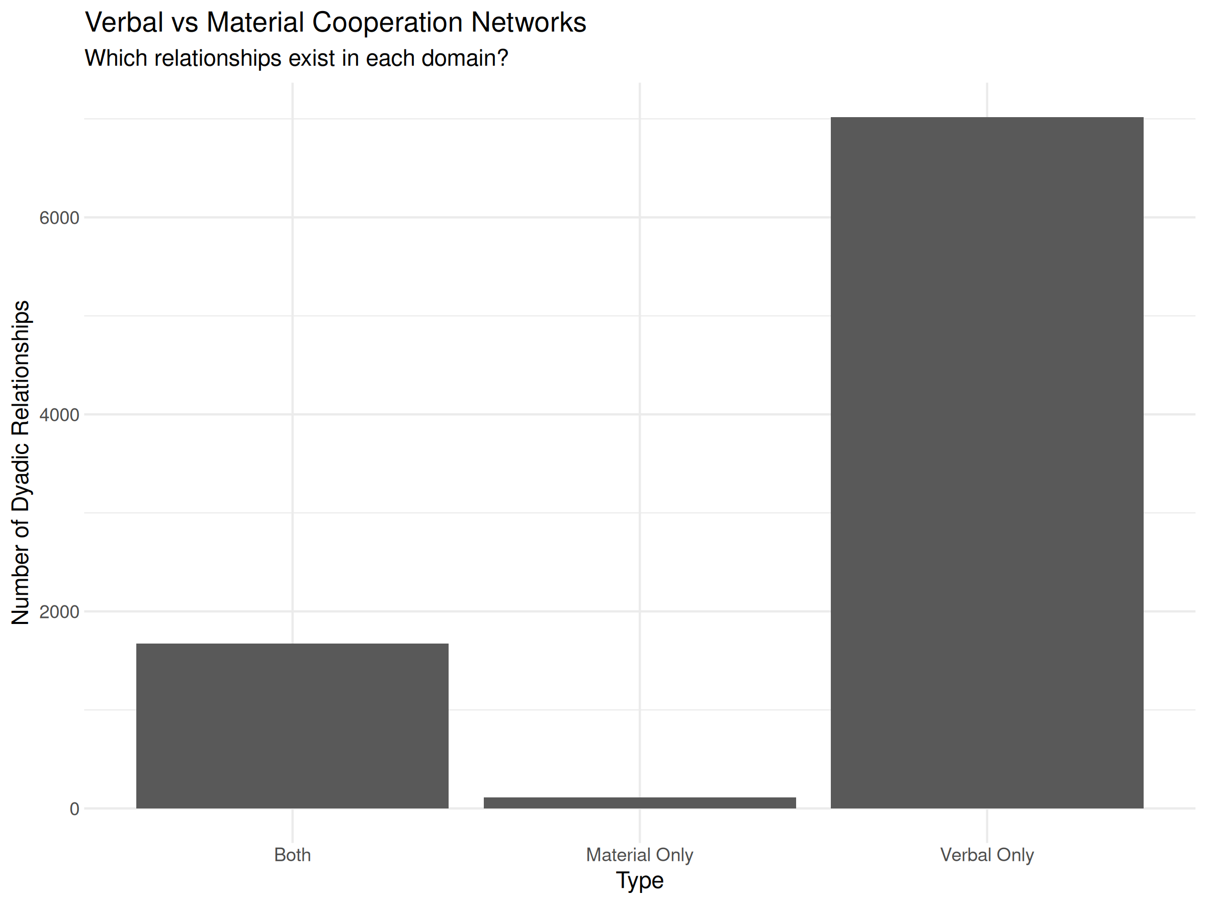
The visualization makes the pattern clear: verbal cooperation (cheap talk) is far more common than material cooperation (costly actions). Note that this pattern may partly reflect reporting bias in event data, as verbal events (statements, promises) are more likely to be captured in news sources than material actions.

2. Cooperation vs. Conflict: Testing Network Relationships

Are cooperation and conflict networks related? Let’s use the QAP (Quadratic Assignment Procedure) method for statistical testing:

# Perform QAP test between cooperation and conflict
coop_conf_qap <- compare_networks(
    list(
        cooperation = verb_coop_2002,
        conflict = verb_conf_2002
    ),
    method = "qap",
    n_permutations = 500, # Reduced for vignette speed
    seed = 12345 # For reproducibility
)

# Construct message
qap_msg <- paste0(
    "**QAP Test Results:**\n\n",
    "- Observed correlation: ", round(coop_conf_qap$summary$qap_correlation, 3), "\n",
    "- P-value: ", ifelse(coop_conf_qap$summary$qap_pvalue == 0, 
                         "< 0.002 (1/500 permutations)", 
                         round(coop_conf_qap$summary$qap_pvalue, 3)), "\n"
)

# Add interpretation based on significance
if (coop_conf_qap$summary$qap_pvalue < 0.05) {
    if (coop_conf_qap$summary$qap_correlation > 0) {
        qap_msg <- paste0(
            qap_msg,
            "→ Cooperation and conflict networks are positively correlated\n",
            "  (Countries interact through both cooperation AND conflict)\n"
        )
    } else {
        qap_msg <- paste0(
            qap_msg,
            "→ Cooperation and conflict networks are negatively correlated\n",
            "  (Different countries engage in cooperation vs conflict)\n"
        )
    }
} else {
    qap_msg <- paste0(
        qap_msg,
        "→ No significant relationship between cooperation and conflict patterns\n"
    )
}

# Print result
cat(qap_msg)

## **QAP Test Results:**
## 
## - Observed correlation: 0.506
## - P-value: < 0.002 (1/500 permutations)
## → Cooperation and conflict networks are positively correlated
##   (Countries interact through both cooperation AND conflict)

Understanding QAP Results

The positive correlation (0.506) with p-value < 0.002 tells us that countries that cooperate also tend to have conflicts. This counterintuitive finding reflects the multiplex nature of international relations: countries that appear frequently in international news tend to have both cooperative and conflictual interactions. High-interaction dyads accumulate both cooperative and conflictual events; the correlation therefore captures activity rather than affinity. In contrast, countries that rarely interact have neither cooperation nor conflict events recorded. This pattern is well-documented in the international relations literature as the “interaction density” effect.

Advanced QAP Options: Different Permutation Schemes

The compare_networks() function supports multiple permutation schemes for more sophisticated hypothesis testing:

# Compare different permutation schemes
qap_methods <- list(
    classic = compare_networks(
        list(cooperation = verb_coop_2002, conflict = verb_conf_2002),
        method = "qap",
        permutation_type = "classic",
        n_permutations = 500,
        seed = 12345
    ),
    freedman_lane = compare_networks(
        list(cooperation = verb_coop_2002, conflict = verb_conf_2002),
        method = "qap",
        permutation_type = "freedman_lane",
        n_permutations = 500,
        seed = 12345
    ),
    dsp_mrqap = compare_networks(
        list(cooperation = verb_coop_2002, conflict = verb_conf_2002),
        method = "qap",
        permutation_type = "dsp_mrqap",
        n_permutations = 500,
        seed = 12345
    )
)

# Compare results
qap_results <- data.frame(
    Permutation_Type = c("Classic", "Freedman-Lane", "DSP-MRQAP"),
    Correlation = c(
        qap_methods$classic$summary$qap_correlation,
        qap_methods$freedman_lane$summary$qap_correlation,
        qap_methods$dsp_mrqap$summary$qap_correlation
    ),
    P_Value = c(
        qap_methods$classic$summary$qap_pvalue,
        qap_methods$freedman_lane$summary$qap_pvalue,
        qap_methods$dsp_mrqap$summary$qap_pvalue
    )
)

knitr::kable(qap_results, 
             caption = "QAP Results with Different Permutation Schemes",
             digits = 3)

QAP Results with Different Permutation Schemes
Permutation_Type	Correlation	P_Value
Classic	0.506	0.000
Freedman-Lane	-0.007	0.112
DSP-MRQAP	-0.007	0.112

Understanding Different Permutation Types:

Classic: Standard node label permutation. Fast and widely used.
Freedman-Lane: Controls for network autocorrelation by residualizing before permutation.
DSP-MRQAP: Double Semi-Partialling - removes mutual influence between networks.

Note that MRQAP methods (Freedman-Lane and DSP) often yield higher p-values as they account for network dependencies. Because Freedman-Lane and DSP residualize the matrices before permutation, the point estimate can shrink and occasionally flip sign; what matters is the (non-)significance after accounting for structural autocorrelation.

Correlation Types: Pearson vs. Spearman

For networks with skewed weight distributions, Spearman correlation may be more appropriate:

# Compare using different correlation types
cor_comparison <- data.frame(
    Correlation_Type = c("Pearson", "Spearman"),
    Cooperation_Networks = c(
        compare_networks(
            list(verbal = verb_coop_2002, material = matl_coop_2002),
            correlation_type = "pearson"
        )$summary$correlation,
        compare_networks(
            list(verbal = verb_coop_2002, material = matl_coop_2002),
            correlation_type = "spearman"
        )$summary$correlation
    ),
    Conflict_Networks = c(
        compare_networks(
            list(verbal = verb_conf_2002, material = matl_conf_2002),
            correlation_type = "pearson"
        )$summary$correlation,
        compare_networks(
            list(verbal = verb_conf_2002, material = matl_conf_2002),
            correlation_type = "spearman"
        )$summary$correlation
    )
)

knitr::kable(cor_comparison,
             caption = "Pearson vs. Spearman Correlations",
             digits = 3)

Pearson vs. Spearman Correlations
Correlation_Type	Cooperation_Networks	Conflict_Networks
Pearson	0.507	0.784
Spearman	0.429	0.535

Spearman correlation is rank-based and more robust to outliers, which is useful when edge weights have extreme values.

3. Temporal Evolution: Tracking Network Changes

How do international networks evolve over time? When you pass a longitudinal netify object to compare_networks(), it automatically compares consecutive time periods:

# Create networks for multiple years
years_to_compare <- seq(2002, 2014, by = 4)

# Create cooperation networks for each year
coop_net_longit <- netify(
    icews[icews$year %in% years_to_compare, ],
    actor1 = "i", actor2 = "j",
    time = "year",
    weight = "verbCoop",
    symmetric = FALSE,
    output_format = "longit_list"
)

# Compare across time - automatic pairwise comparisons
temporal_comparison <- compare_networks(
    coop_net_longit,
    method = "all"
)
# Display temporal comparison results
# Show summary statistics in a cleaner format
knitr::kable(
    temporal_comparison$summary,
    caption = "Temporal Network Comparison Summary",
    digits = 3,
    align = "c"
)

Temporal Network Comparison Summary
metric	mean	sd	min	max
correlation	0.828	0.034	0.771	0.874
jaccard	0.581	0.014	0.561	0.594
hamming	0.217	0.009	0.200	0.225
spectral	13325.806	3718.830	9436.173	18155.052

Understanding Temporal Comparison Output

Header Changes:

Type: temporal - Indicates we’re comparing time periods from the same longitudinal network
Networks compared: 4 - We have 4 time periods (2002, 2006, 2010, 2014)

Summary Statistics Table:

Instead of a single comparison, we see summary statistics across ALL pairwise comparisons:

mean correlation (0.828): On average, networks are highly correlated across time
sd (0.034): Very low standard deviation indicates consistent similarity
min (0.771) to max (0.874): Even the least similar pair of years has correlation > 0.77

This high correlation tells us that cooperation networks are quite stable over time - the same countries tend to cooperate across years.

Edge Changes Section:

Shows all pairwise comparisons (not just consecutive years):

2002_vs_2006: First comparison
2010_vs_2014: Last consecutive comparison
Notice that as time gaps increase, more edges are added/removed

Visualizing Temporal Changes

# Extract edge changes over time
edge_change_data <- data.frame(
    Comparison = names(temporal_comparison$edge_changes),
    Added = sapply(temporal_comparison$edge_changes, function(x) x$added),
    Removed = sapply(temporal_comparison$edge_changes, function(x) x$removed),
    Maintained = sapply(temporal_comparison$edge_changes, function(x) x$maintained)
)

# Reshape for plotting
edge_change_long <- edge_change_data %>%
    pivot_longer(
        cols = c(Added, Removed, Maintained),
        names_to = "Change_Type",
        values_to = "Count"
    )

# Plot edge changes
ggplot(edge_change_long, aes(x = Comparison, y = Count, fill = Change_Type)) +
    geom_col(position = "dodge") +
    scale_fill_manual(
        values = c(
            "Added" = "#A8D5BA",
            "Removed" = "#E8B4B8",
            "Maintained" = "#95A99C"
        )
    ) +
    labs(
        title = "Edge Changes Between Years",
        subtitle = "Tracking relationship dynamics over time",
        x = "Year Comparison",
        y = "Number of Edges"
    ) +
    theme_minimal() +
    theme(
        axis.text.x = element_text(
            angle = 45, hjust = 1
        )
    )

Notice that “Maintained” edges dominate - most relationships persist across time periods, confirming the stability we observed in the correlation metrics.

Multiple Testing Correction

When comparing multiple networks, it’s important to adjust p-values for multiple comparisons. The p_adjust parameter offers several correction methods:

# Demonstrate multiple testing correction
# Compare all years pairwise with QAP
multi_year_comparison <- compare_networks(
    coop_net_longit,
    method = "qap",
    n_permutations = 500,  # Lower for vignette
    p_adjust = "BH",  # Benjamini-Hochberg correction
    seed = 123
)

# Show adjusted p-values
cat("Number of pairwise comparisons:", 
    choose(length(names(coop_net_longit)), 2), "\n")

## Number of pairwise comparisons: 6

cat("P-value adjustment method: Benjamini-Hochberg (FDR)\n\n")

## P-value adjustment method: Benjamini-Hochberg (FDR)

# Display the p-value matrix
knitr::kable(
    round(multi_year_comparison$significance_tests$qap_pvalues, 4),
    caption = "QAP P-values (Adjusted using BH method)",
    align = "c"
)

QAP P-values (Adjusted using BH method)
	2002	2006	2010	2014
2002	0	0	0	0
2006	0	0	0	0
2010	0	0	0	0
2014	0	0	0	0

Available p-value adjustment methods:

"none": No adjustment (default)
"holm": Holm’s method (controls family-wise error rate)
"BH": Benjamini-Hochberg (controls false discovery rate)
"BY": Benjamini-Yekutieli (more conservative FDR control)

Use p-value adjustment when making many comparisons to avoid inflated Type I error rates.

4. Structural Evolution: Beyond Individual Edges

The what = "structure" option compares network-level properties rather than individual edges:

# Compare structural properties across years
struct_comparison <- compare_networks(
    coop_net_longit,
    what = "structure"
)

# Display structural comparison
knitr::kable(struct_comparison$summary,
    caption = "Structural Properties Across Time Periods",
    digits = 3,
    align = "c"
)

Structural Properties Across Time Periods
network	n_nodes	n_edges	density	reciprocity	transitivity	mean_degree
2002	152	8692	0.376	0.978	0.606	57.184
2006	152	9429	0.408	0.977	0.628	62.033
2010	152	9976	0.432	0.982	0.639	65.632
2014	152	9774	0.423	0.973	0.630	64.303

Understanding Structural Comparison Output

This table shows how network-wide properties evolve:

n_nodes (152): Number of countries remains constant - same actors throughout
n_edges: Increases from 8,692 (2002) to 9,774 (2014) - more connections over time
density: Increases from 0.376 to 0.423 - the network becomes denser
reciprocity: Stays very high (0.97-0.98) - if country A cooperates with B, B almost always cooperates with A
transitivity: Around 0.61-0.64 - moderate clustering (friend of a friend is often a friend)
mean_degree: Increases from 57.2 to 64.3 - average country has more partners over time

The increasing density and mean degree suggest growing interconnectedness in international cooperation.

Visualizing Structural Changes

# Prepare data for visualization
# struct_comparison$summary contains a
# data.frame with structural metrics over time
struct_data <- struct_comparison$summary

# Calculate percent changes from baseline
baseline_year <- struct_data$network[1]
struct_long <- struct_data %>%
    select(-n_nodes) %>% # Remove n_nodes since it doesn't change much
    pivot_longer(cols = -network, names_to = "metric", values_to = "value") %>%
    group_by(metric) %>%
    mutate(
        first_value = value[1],
        percent_change = (value - first_value) / first_value * 100
    ) %>%
    ungroup()

# Create heatmap of changes
ggplot(
    filter(struct_long, network != baseline_year),
    aes(x = network, y = metric, fill = percent_change)
) +
    geom_tile(color = "white") +
    geom_text(aes(label = round(percent_change, 1)), color = "black", size = 4) +
    scale_fill_gradient2(
        low = "#d73027", mid = "white", high = "#1a9850",
        midpoint = 0, name = "% Change"
    ) +
    labs(
        title = "Structural Changes Heatmap",
        subtitle = paste("Percent change from", baseline_year),
        x = "", y = ""
    ) +
    theme_minimal() +
    theme(axis.text.x = element_text(angle = 0))

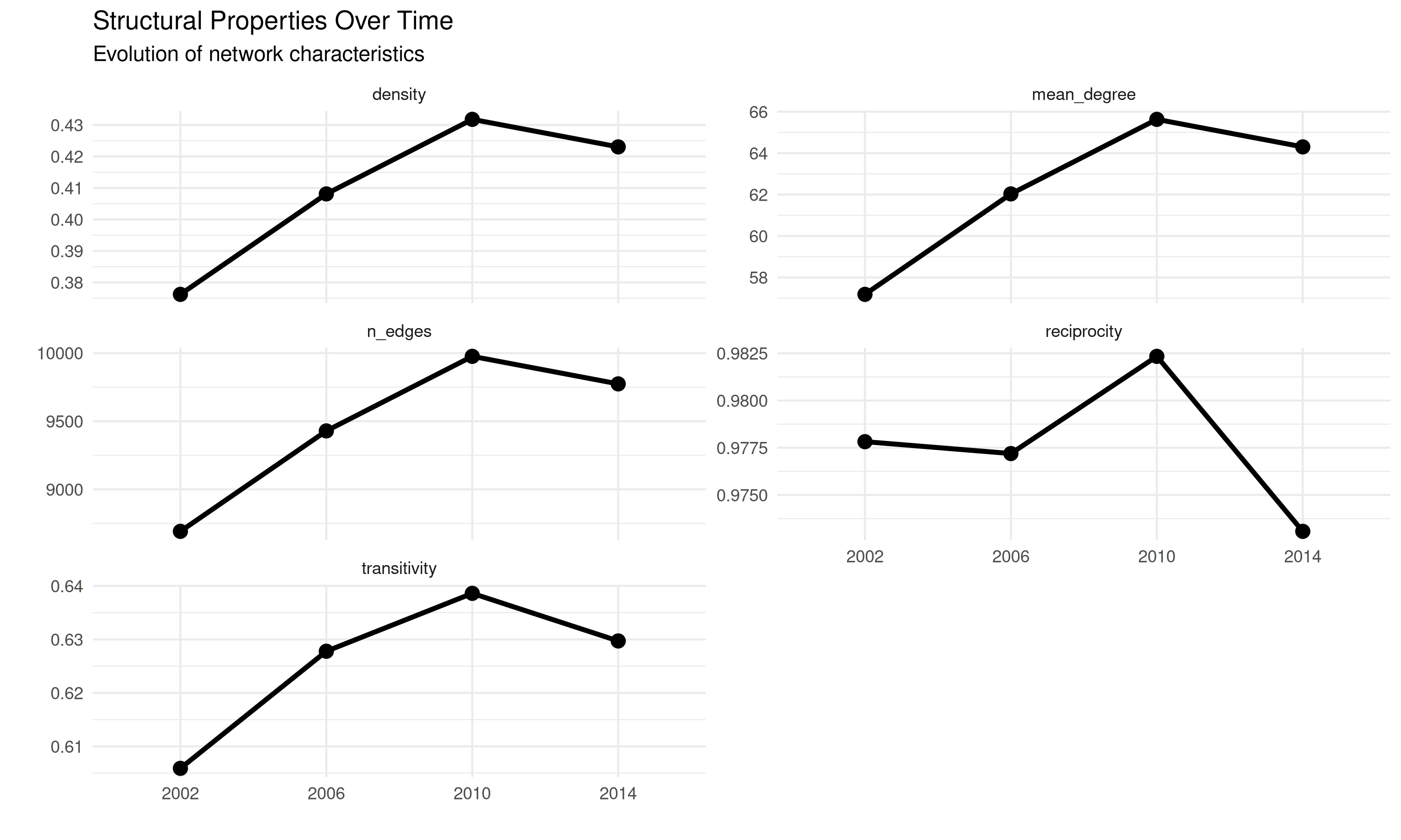
The heatmap reveals that density, number of edges, and mean degree all increase by about 14-15% from 2002 to 2010, while reciprocity slightly decreases and transitivity shows modest growth.

Many ways to visualize structural changes … could also just do a line plot:

# Reshape data for visualization
struct_long <- struct_data %>%
    select(-n_nodes) %>% # Remove n_nodes since it doesn't change
    pivot_longer(cols = -network, names_to = "metric", values_to = "value") %>%
    group_by(metric) %>%
    mutate(
        # Calculate percent change from first year
        first_value = value[1],
        percent_change = (value - first_value) / first_value * 100,
        # Also calculate year-to-year change
        yoy_change = (value - lag(value)) / lag(value) * 100
    ) %>%
    ungroup()

# Visualize structural changes over time
ggplot(struct_long, aes(x = network, y = value, group = metric)) +
    geom_line(size = 1.2) +
    geom_point(size = 3) +
    facet_wrap(~metric, scales = "free_y", ncol = 2) +
    labs(
        title = "Structural Properties Over Time",
        subtitle = "Evolution of network characteristics",
        x = "", y = ""
    ) +
    theme_minimal() +
    theme(legend.position = "none")

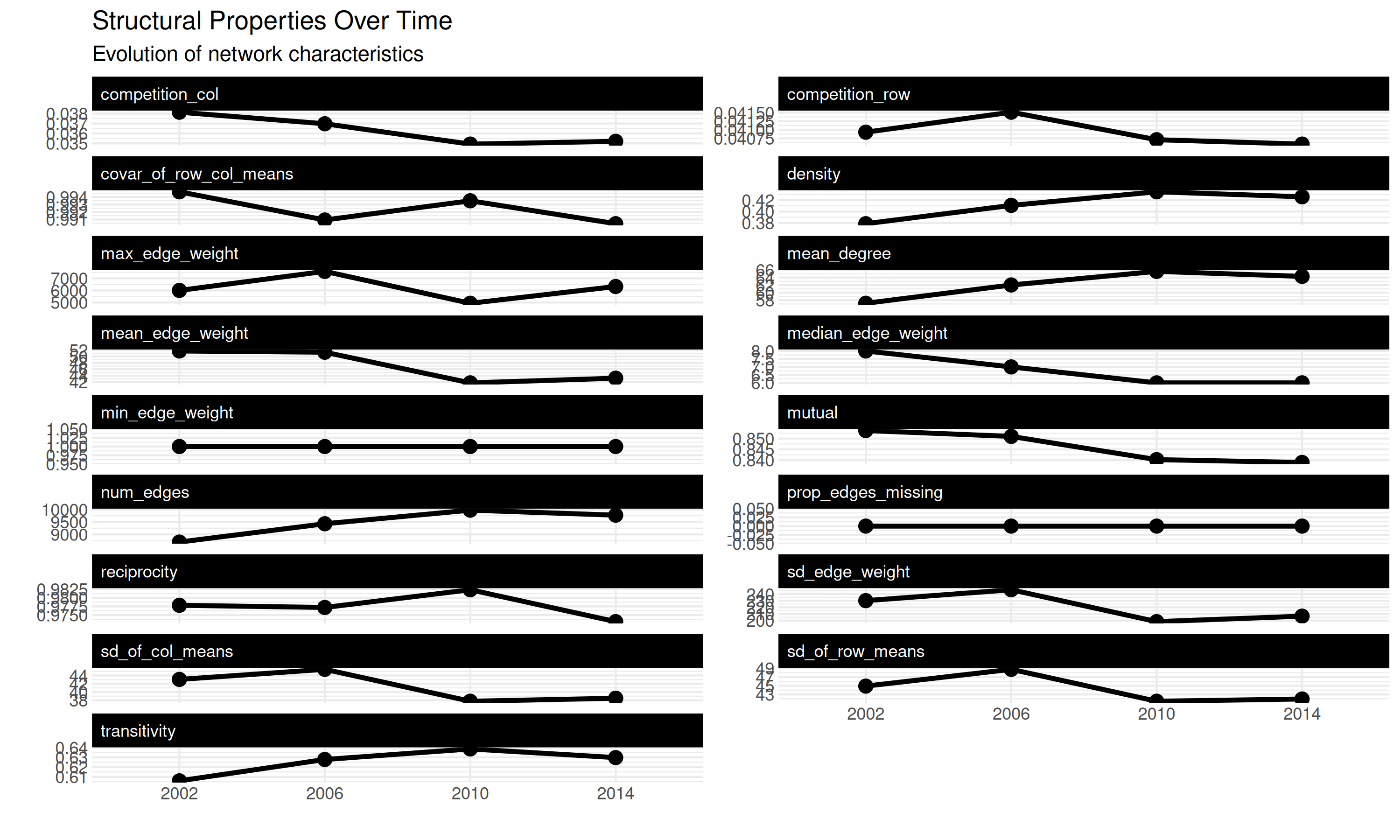
5. Node Composition: Tracking Actor Dynamics

The what = "nodes" option tracks which actors enter and exit the network:

# Compare node composition
node_comparison <- compare_networks(
    coop_net_longit,
    what = "nodes"
)

# Display node comparison
knitr::kable(node_comparison$summary,
    caption = "Node Composition Across Time Periods",
    digits = 0,
    align = "c",
    row.names = FALSE
)

Node Composition Across Time Periods
network	n_nodes	mean_overlap	mean_jaccard
2002	152	152	1
2006	152	152	1
2010	152	152	1
2014	152	152	1

The table shows:

All networks have 152 nodes (countries)
mean_overlap = 152: All 152 countries appear in all comparisons

This is by design in our example since we filtered the data to only include certain countries. In real-world datasets, you might see actors entering or exiting the network over time.

6. Deep Dive: Using return_details for Comprehensive Analysis

The return_details = TRUE option provides access to full comparison matrices:

# Compare 2002 and 2014 cooperation networks with full details
early_late_comp <- compare_networks(
    # note subset here is
    # subset.netify() function
    subset(
        coop_net_longit,
        time = c("2002", "2014")
    ),
    method = "all",
    return_details = TRUE,
    n_permutations = 1000 # Lower for vignette speed
)

# Access detailed comparison matrices
names(early_late_comp$details)

## [1] "correlation_matrix" "jaccard_matrix"     "hamming_matrix"    
## [4] "spectral_matrix"

# Get edge changes
changes <- early_late_comp$edge_changes[[1]]

# Summary of relationship dynamics
changes_summary <- paste0(
    "**Relationship Dynamics 2002-2014:**\n\n",
    "- Stable relationships: ", changes$maintained, "\n",
    "- New relationships: ", changes$added, "\n",
    "- Ended relationships: ", changes$removed, "\n",
    "- Total change rate: ",
    round((changes$added + changes$removed) /
        (changes$maintained + changes$added + changes$removed) * 100, 1), "%\n"
)

if (!is.na(changes$weight_correlation)) {
    changes_summary <- paste0(
        changes_summary,
        "- Weight correlation for maintained edges: ",
        round(changes$weight_correlation, 3), "\n"
    )

    if (changes$weight_correlation > 0.7) {
        changes_summary <- paste0(
            changes_summary,
            "  → Stable cooperation intensities for continuing relationships\n"
        )
    } else {
        changes_summary <- paste0(
            changes_summary,
            "  → Cooperation intensities vary even for maintained relationships\n"
        )
    }
}

Relationship Dynamics 2002-2014:

Stable relationships: 6633
New relationships: 3141
Ended relationships: 2059
Total change rate: 43.9%
Weight correlation for maintained edges: 0.762 → Stable cooperation intensities for continuing relationships

Understanding Detailed Output

With return_details = TRUE, you get:

Access to full similarity matrices (correlation_matrix, jaccard_matrix, hamming_matrix)
These allow custom analysis and visualization of network similarities

The relationship dynamics show:

6,633 stable relationships persist from 2002 to 2014
3,141 new relationships formed
2,059 relationships ended
43.9% total change rate indicates moderate network evolution
Weight correlation of 0.762 means cooperation intensity is fairly stable for continuing relationships

With this detailed information you could create custom visualizations or further statistical tests, such as detecting structural breaks in time series.

7. Spectral Distance: Comparing Network Structure Through Eigenvalues

The spectral distance approach provides a way to compare networks based on their fundamental structural properties captured by eigenvalues (See Shimada et al 2016 for a useful introduction):

# Compare networks using spectral distance
spectral_comp <- compare_networks(
    list(
        "2002" = coop_net_longit[["2002"]],
        "2014" = coop_net_longit[["2014"]]
    ),
    method = "spectral"
)

# Display spectral comparison results in a cleaner format
knitr::kable(
    spectral_comp$summary,
    caption = "Spectral Distance Results",
    digits = 2,
    align = "c"
)

Spectral Distance Results
comparison	spectral
2002 vs 2014	14369.14

# Interpretation
# Build spectral interpretation message
spec_dist <- spectral_comp$summary$spectral

spec_msg <- paste0(
    "**SPECTRAL DISTANCE INTERPRETATION**\n\n",
    "- Spectral distance: ", round(spec_dist, 2), "\n"
)

# Add interpretation
# Note: Spectral distance should be interpreted relative to other comparisons
# in your study, as the scale depends on network size
interpretation <- paste0(
    "→ The spectral distance of ", round(spec_dist, 0), 
    " should be interpreted relative to other network comparisons in your study.\n",
    "  Larger values indicate greater structural differences."
)

# Combine and print
cat(paste0(spec_msg, "→ ", interpretation))

## **SPECTRAL DISTANCE INTERPRETATION**
## 
## - Spectral distance: 14369.14
## → → The spectral distance of 14369 should be interpreted relative to other network comparisons in your study.
##   Larger values indicate greater structural differences.

Understanding Spectral Distance

Spectral distance measures how different two networks are by comparing their eigenvalue spectra. It captures global structural properties that other metrics might miss:

What it measures: The distance between the sorted eigenvalues of two network Laplacian matrices
Scale: Ranges from 0 (identical spectra) to potentially large values depending on network size
Advantages:
- Captures global network structure
- Sensitive to community structure and clustering patterns
- Robust to node relabeling
Use cases:
- Detecting fundamental structural changes over time
- Comparing networks with different connectivity patterns
- Identifying networks with similar spectral properties (useful for network classification)

Performance Optimization for Large Networks

For large networks (>1000 nodes), computing all eigenvalues can be computationally expensive. The spectral_rank parameter allows you to use only the top-k eigenvalues:

# For large networks, use spectral_rank to improve performance
spectral_comp_fast <- compare_networks(
    list(large_net1, large_net2),
    method = "spectral",
    spectral_rank = 50  # Use only top 50 eigenvalues (rule of thumb: round(sqrt(n)))
)

The top eigenvalues capture the most significant structural features. A good rule of thumb is to use round(sqrt(n)) eigenvalues, where n is the number of nodes.

Combining with Other Methods

# Compare all methods including spectral
full_comp <- compare_networks(
    list(
        early = coop_net_longit[["2002"]],
        late = coop_net_longit[["2014"]]
    ),
    method = "all",
    return_details = TRUE
)

# Extract similarity metrics (0-1 scale) and spectral distance separately
similarity_metrics <- data.frame(
    Method = c("Correlation", "Jaccard", "Hamming"),
    Value = c(
        full_comp$summary$correlation,
        full_comp$summary$jaccard,
        full_comp$summary$hamming
    )
)

spectral_distance <- full_comp$summary$spectral

# Display similarity metrics table
knitr::kable(
    rbind(
        similarity_metrics,
        data.frame(Method = "Spectral Distance", Value = spectral_distance)
    ),
    caption = "Network Similarity Metrics: 2002 vs 2014",
    digits = 3,
    align = "c"
)

Network Similarity Metrics: 2002 vs 2014
Method	Value
Correlation	0.771
Jaccard	0.561
Hamming	0.225
Spectral Distance	14369.141

# Create visualization for similarity metrics
p_similarity <- ggplot(similarity_metrics, aes(x = Method, y = Value)) +
    geom_col(fill = "gray30", width = 0.7) +
    geom_text(aes(label = round(Value, 3)), hjust = -0.1, size = 3.5) +
    scale_y_continuous(limits = c(0, 1.1), breaks = seq(0, 1, 0.2)) +
    labs(
        title = "Similarity Metrics (0-1 Scale)",
        x = NULL, y = "Similarity Score"
    ) +
    theme_minimal() +
    coord_flip()

# Create separate note for spectral distance
spectral_note <- paste("Spectral Distance:", round(spectral_distance, 2))

# Combine the plot with spectral distance information
library(patchwork)
p_similarity + plot_annotation(
    title = "Network Comparison: Multiple Metrics",
    subtitle = paste("2002 vs 2014 Cooperation Networks |", spectral_note),
    theme = theme(plot.title = element_text(face = "bold"))
)

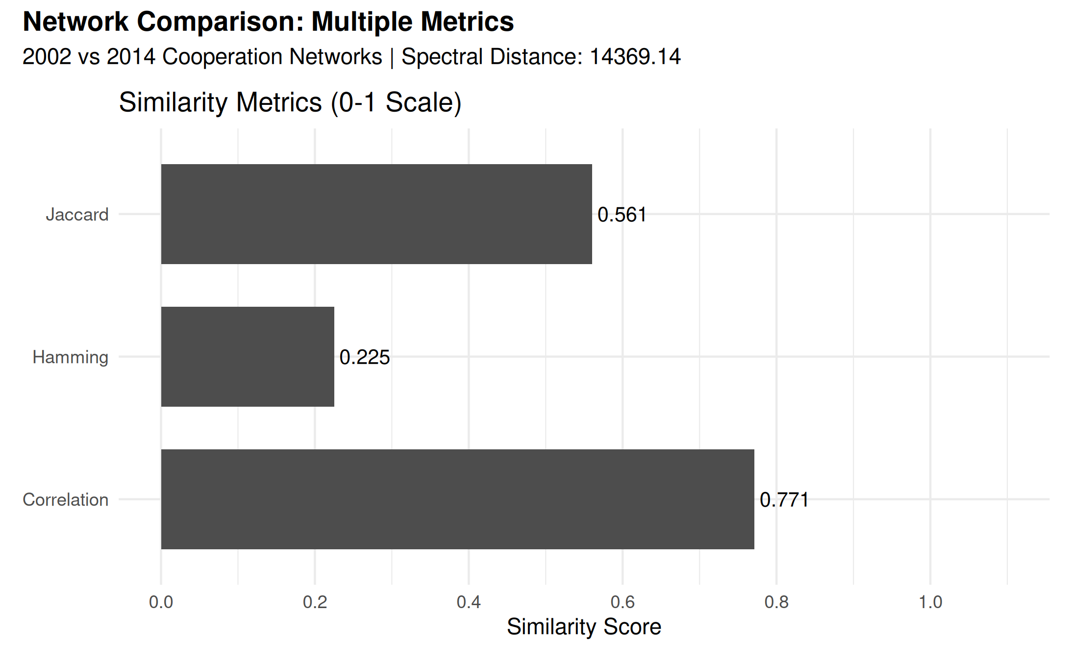
Note that spectral distance is on a different scale than the other metrics (which are typically 0-1), so it’s best interpreted relative to other spectral distance values rather than in absolute terms.

8. Multilayer Networks: Comparing Different Relationship Types

The compare_networks() function automatically handles multilayer networks created with layer_netify(). This allows you to compare different types of relationships (layers) within the same set of actors:

# Create multilayer network for 2010
icews_2010 <- icews[icews$year == 2010, ]

# Create individual networks for each layer
verb_coop_2010 <- netify(
    icews_2010,
    actor1 = "i", actor2 = "j",
    weight = "verbCoop",
    symmetric = FALSE
)

matl_coop_2010 <- netify(
    icews_2010,
    actor1 = "i", actor2 = "j",
    weight = "matlCoop",
    symmetric = FALSE
)

verb_conf_2010 <- netify(
    icews_2010,
    actor1 = "i", actor2 = "j",
    weight = "verbConf",
    symmetric = FALSE
)

matl_conf_2010 <- netify(
    icews_2010,
    actor1 = "i", actor2 = "j",
    weight = "matlConf",
    symmetric = FALSE
)

# Combine into multilayer network
multilayer_2010 <- layer_netify(
    list(
        verbal_coop = verb_coop_2010,
        material_coop = matl_coop_2010,
        verbal_conf = verb_conf_2010,
        material_conf = matl_conf_2010
    )
)

# Compare layers automatically
layer_comparison <- compare_networks(multilayer_2010, method = "all")
# Display multilayer comparison results
# Extract summary for cleaner display
knitr::kable(
    layer_comparison$summary,
    caption = "Multilayer Network Comparison Summary",
    digits = 3,
    align = "c"
)

Multilayer Network Comparison Summary
metric	mean	sd	min	max
correlation	0.531	0.106	0.422	0.643
jaccard	0.280	0.069	0.198	0.385
hamming	0.223	0.129	0.100	0.351
spectral	42200.921	42019.957	529.314	84148.029

Understanding Multilayer Comparison Output

When you pass a multilayer network to compare_networks(), it automatically:

Detects that it’s a multilayer network (Type: multilayer)
Extracts each layer for comparison
Performs pairwise comparisons between all layers

The output shows how different types of relationships relate to each other. For example:

High correlation between verbal and material cooperation suggests consistency across cooperation types
Lower correlation between cooperation and conflict layers indicates these are distinct relationship patterns

Interpreting Multilayer Results

The output shows all pairwise comparisons between the four network layers. Key insights:

Cooperation vs. Conflict: Verbal cooperation has the highest correlation with verbal conflict (0.628), suggesting countries that cooperate verbally also engage in verbal conflicts
Verbal vs. Material: Within cooperation types, verbal and material cooperation are moderately correlated (0.587)
Cross-type patterns: Material cooperation shows lower correlation with conflict types, indicating material actions may be more distinct from conflict behaviors

The summary statistics show correlations range from 0.42 to 0.64 across all layer pairs, indicating moderate but meaningful relationships between different interaction types.

Longitudinal Multilayer Networks

You can also compare multilayer networks that evolve over time:

# Create longitudinal multilayer networks
verb_coop_longit <- netify(
    icews,
    actor1 = "i", actor2 = "j",
    time = "year",
    weight = "verbCoop",
    symmetric = FALSE,
    output_format = "longit_array"
)

matl_coop_longit <- netify(
    icews,
    actor1 = "i", actor2 = "j",
    time = "year",
    weight = "matlCoop",
    symmetric = FALSE,
    output_format = "longit_array"
)

# Combine into longitudinal multilayer
longit_multilayer <- layer_netify(
    list(
        verbal = verb_coop_longit,
        material = matl_coop_longit
    )
)

# Compare layers across all time periods
longit_layer_comp <- compare_networks(longit_multilayer)

# Display results cleanly
longit_summary <- paste0(
    "**Longitudinal multilayer comparison:**\n\n",
    "- Type: ", longit_layer_comp$comparison_type, "\n",
    "- Number of layers compared: ", longit_layer_comp$n_networks, "\n",
    "- Average correlation between verbal and material cooperation: ",
    round(mean(longit_layer_comp$summary$correlation), 3), "\n"
)

Longitudinal multilayer comparison:

Type: multilayer
Number of layers compared: 2
Average correlation between verbal and material cooperation: 0.507

This shows how the relationship between different types of cooperation remains stable or changes over time.

tl;dr

The compare_networks() function is your go-to tool for understanding how networks differ and change:

Basic usage:

# Compare two networks
comparison <- compare_networks(list(net1, net2))

# Compare longitudinal networks automatically
comparison <- compare_networks(longitudinal_netify_object)

Key parameters to remember:

method: “correlation” (default), “jaccard”, “hamming”, “qap”, “spectral”, or “all”
what: “edges” (default), “structure”, “nodes”, or “attributes”
return_details: Set TRUE to get full comparison matrices
n_permutations: For QAP significance testing (default 5000)
permutation_type: “classic” (default), “degree_preserving”, “freedman_lane”, or “dsp_mrqap”
correlation_type: “pearson” (default) or “spearman”
seed: Set for reproducible permutation tests
p_adjust: “none” (default), “holm”, “BH”, or “BY” for multiple testing correction
spectral_rank: Number of eigenvalues for spectral distance (0 = all, default). Rule of thumb: round(sqrt(n)) for networks with many nodes

What you get:

Summary statistics: Correlation, Jaccard similarity, Hamming distance, spectral distance
Edge changes: Detailed counts of added, removed, and maintained edges
Statistical tests: Permutation tests for significance
Flexible comparisons: Works with any number of networks, automatically handles longitudinal data

Use method = "all" for initial exploration
Use what = "structure" to compare network-level properties
Set return_details = TRUE when you need the full comparison matrices
For longitudinal data, just pass your netify object - it handles the rest
Use permutation_type = "freedman_lane" or "dsp_mrqap" when comparing networks that may have autocorrelation
Set correlation_type = "spearman" for networks with skewed weight distributions
Use p_adjust when making multiple comparisons to control false discovery rate
Set spectral_rank = round(sqrt(n)) for large networks to improve performance

When to Use Advanced Options

The compare_networks() function includes several advanced parameters that help tailor the analysis to your specific network characteristics:

Permutation Types:

classic (default): Standard node label permutation. Use for general network comparisons.
degree_preserving: Maintains degree sequences through edge swaps. Essential for sparse, binary networks with high degree heterogeneity.
freedman_lane: Residualizes before permutation. Use when you suspect network autocorrelation (e.g., geographic networks, social influence).
dsp_mrqap: Double semi-partialling. Most conservative option; use for multiple regression-style comparisons or when networks have strong mutual dependencies.

Correlation Types:

pearson (default): Standard linear correlation. Appropriate for normally distributed edge weights.
spearman: Rank-based correlation. Use when edge weights are skewed, zero-inflated, or contain outliers.

P-value Adjustments:

none (default): No adjustment. Fine for single comparisons.
holm: Controls family-wise error rate. Use for a small number of planned comparisons.
BH (Benjamini-Hochberg): Controls false discovery rate. Best for many comparisons (e.g., comparing all time periods).
BY (Benjamini-Yekutieli): More conservative FDR control. Use when comparisons are strongly dependent.

Binary Metrics (for binary networks):

phi: Phi coefficient. Standard choice, but sensitive to marginal imbalance.
simple_matching: Proportion of matching edges. Use when absence of edges is as meaningful as presence.
mean_centered: Centers matrices before correlation. Reduces bias from density differences.

Using `compare_networks()` in Your Research Workflow

Where `compare_networks()` Fits in Network Analysis

The compare_networks() function serves as a comprehensive diagnostic tool that should be used throughout your network analysis workflow:

Analysis Stage	Key Questions	How `compare_networks()` Helps
Data cleaning	Have I built the networks correctly?	Quick edge & node sanity checks
Exploration	Where are the major differences?	Multi-metric similarity diagnostics
Theory building	Which dimensions matter (time, layer, subgroup)?	Temporal/multilayer/by-group comparisons highlight mechanisms
Model specification	Which terms belong in my ERGM/SAOM?	Structural summaries reveal relevant patterns
Model validation	Does my model capture observed differences?	Compare observed vs. simulated networks

Recommended Pre-Modeling Workflow

Before fitting ERGMs, SAOMs, or latent space models, follow this systematic approach:

Sanity Check: compare_networks(nets, method="all", what="edges")
- Identify duplicate edges, missing dyads, density anomalies
- Clean data or adjust netify() parameters as needed
Cross-Domain Analysis: Compare different relationship types
- Example: verbal vs. material cooperation
- Decides whether to model layers jointly (multiplex ERGM) or separately
Temporal Stability: compare_networks(longit_nets, method="all")
- How quickly do ties appear/disappear?
- Informs SAOM rate functions or ERGM temporal windows
Actor Dynamics: compare_networks(nets, what="nodes")
- Track actor turnover
- Choose between relational event models vs. panel frameworks
Structural Evolution: compare_networks(nets, what="structure")
- Identify density, reciprocity, transitivity trends
- Suggests candidate ERGM terms or SAOM effects
Global Shifts: compare_networks(nets, method="spectral")
- Detect regime-change style discontinuities
- May require sample breaks or change-point models
Statistical Validation: compare_networks(nets, method="qap", permutation_type="...")
- Test if correlations are spurious under network constraints
- Guides which controls must enter your model

Interpreting Results for Model Building

For ERGMs:

High transitivity → include GWESP terms
Degree heterogeneity → add degree-based terms (e.g., gwidegree)
Reciprocity changes → include mutual edge terms
Spectral distance jumps → consider time-varying parameters

For SAOMs:

Edge turnover rates → set appropriate rate functions
Structural stability → choose evaluation vs. creation effects
Actor composition changes → include composition change effects

For Latent Space Models:

Spectral distance magnitude → suggests latent dimensionality
Community structure (from eigenvalues) → number of latent positions
Temporal stability → fixed vs. dynamic latent positions

Computational Considerations

For large networks (>1000 nodes):

Set spectral_rank = round(sqrt(n)) for faster spectral comparisons
Use n_permutations = 1000 for initial exploration, increase for final analysis
Consider correlation_type = "spearman" for heavy-tailed weight distributions
Always use p_adjust when making many comparisons

Example: Complete Pre-Modeling Diagnostic

# Comprehensive diagnostic before ERGM fitting
diagnostic_results <- compare_networks(
    network_list,
    method = "all",
    what = "edges",
    permutation_type = "degree_preserving",  # For sparse networks
    correlation_type = "spearman",           # For skewed weights
    n_permutations = 10000,                  # For publication
    p_adjust = "BH",                         # Multiple comparisons
    spectral_rank = 75,                      # Large network optimization
    return_details = TRUE,                   # For custom analysis
    seed = 12345                             # Reproducibility
)

# Extract insights for model specification
if (diagnostic_results$summary$transitivity > 0.3) {
    # High clustering suggests including triadic closure terms
    ergm_formula <- formula(net ~ edges + gwesp(0.5, fixed=TRUE))
}

if (diagnostic_results$spectral > 100) {
    # Large spectral distance suggests structural regime change
    # Consider separate models for different periods
}

Metric Interpretation Guidelines

Edge-level Metrics:

Correlation (-1 to 1): Linear association between edge weights
- 0.7+ = Strong alignment
- 0.4-0.7 = Moderate relationship
- <0.4 = Weak or specialized overlap
Jaccard (0 to 1): Proportion of dyads that appear in at least one of the two networks that appear in both
- Context-dependent: 0.25 is high for sparse international relations data
- 0.5+ indicates substantial structural similarity
Hamming (0 to 1): Proportion of dyads that differ
- The denominator is the count of dyads observed in both matrices after NA handling
- 0.2 = 20% edge turnover (moderate change)
- 0.5+ = Major restructuring
Spectral Distance: No fixed scale; interpret relatively
- Doubling from baseline often indicates structural regime change
- Compare within same study/time period

QAP p-values:

Interpret conditional on permutation engine used
degree_preserving typically more conservative than classic
Small p-values more credible with more permutations

Computational Performance Guide

Method	Time Complexity	Memory Usage	When to Optimize
Correlation	O(n²)	Low	Rarely needed
Jaccard/Hamming	O(n²)	Low	Rarely needed
Spectral	O(n³)	O(n²)	Use `spectral_rank` for n>1000
QAP Classic	O(R×n²)	Moderate	Reduce permutations for exploration
QAP Degree-Preserving	O(R×m)	High	Most expensive; use selectively

R = number of permutations, n = number of nodes, m = number of edges

Common Pitfalls and Solutions

Binary vs. Weighted Networks
- If your “weighted” network is actually binary (0/1), set binary_metric appropriately
- Different density networks need binary_metric = "simple_matching"
Temporal Comparisons
- Always check actor composition first with what = "nodes"
- High node turnover invalidates edge-level comparisons
Multiple Testing
- With 10+ comparisons, always use p_adjust
- Report both raw and adjusted p-values in publications
Reproducibility
- Always set seed for permutation tests
- The function captures and reports the seed used

The compare_networks() function is your comprehensive pre-modeling diagnostic tool. Use it early and often to ensure your subsequent modeling choices are well-informed and defensible.

Cassy Dorff and Shahryar Minhas

2025-06-30