Pipeline: netify to lame and dbn

Latent space models for network data require array inputs that are easy to get wrong by hand. The amen package handles cross-sectional and single-layer longitudinal networks, lame adds support for longitudinal networks with changing actor sets, and dbn fits Dynamic Bilinear Network models to multilayer longitudinal networks. Each package expects a different shape: 3D arrays, lists of matrices, or 4D arrays. netify() and layer_netify() build the network object; to_amen(), to_lame(), and to_dbn() export the shape needed by the modeling package.

The conversion chunks use netify. The model-fitting chunks require lame or dbn; install those packages before running them. You can still run the conversion chunks to inspect the arrays that netify creates.

setup

The examples below use ICEWS event data, which captures directed interactions between 152 countries from 2002 to 2014 across four relation types: verbal cooperation, material cooperation, verbal conflict, and material conflict.

library(netify)
library(ggplot2)

# load the icews event data
data(icews)

# preview
head(icews[, c("i", "j", "year", "verbCoop", "matlCoop", "verbConf", "matlConf")], 4)
#>             i       j year verbCoop matlCoop verbConf matlConf
#> 2 Afghanistan Albania 2002        6        1        0        0
#> 3 Afghanistan Albania 2003        1        1        0        0
#> 4 Afghanistan Albania 2004       10        2        0        1
#> 5 Afghanistan Albania 2005        0        0        0        0

part 1: single-layer pipeline (netify to amen)

step 1: create the network

The first step is always netify(). We create a single directed, weighted network representing verbal cooperation over time.

verbal_net = netify(
    icews,
    actor1 = "i", actor2 = "j", time = "year",
    symmetric = FALSE,
    weight = "verbCoop",
    missing_to_zero = FALSE,
    nodal_vars = c("i_polity2", "i_log_gdp"),
    dyad_vars = c("matlCoop", "verbConf"),
    dyad_vars_symmetric = c(FALSE, FALSE),
    output_format = "longit_array"
)

verbal_net

Key choices:

missing_to_zero = FALSE: Preserving NAs distinguishes “no observed interaction” from “structurally impossible interaction.” This matters for latent space models where missing data and structural zeros have different likelihoods.
output_format = "longit_array": We use array format because our actor set is constant across time.
nodal_vars and dyad_vars: These covariates will be carried through to the amen output automatically.

step 2: inspect the network

Before modeling, it’s worth checking basic properties.

# quick summary
net_summary = summary(verbal_net)
head(net_summary[, c("net", "num_actors", "density", "num_edges", "reciprocity")])
#>    net num_actors   density num_edges reciprocity
#> 1 2002        152 0.3787034      8692   0.9778217
#> 2 2003        152 0.3871994      8887   0.9632488
#> 3 2004        152 0.4145173      9514   0.9769563
#> 4 2005        152 0.4071976      9346   0.9804325
#> 5 2006        152 0.4108139      9429   0.9771928
#> 6 2007        152 0.4243203      9739   0.9783703

# visualize a single year
verbal_2010 = subset(verbal_net, time = "2010")
plot(verbal_2010, add_text = FALSE)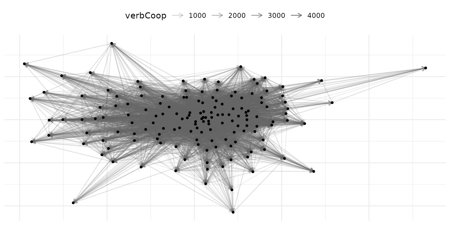

step 3: convert to amen format

to_amen() converts a single-layer netify object into the list structure that amen::ame() expects.

amen_data = to_amen(verbal_net)

# inspect the resulting array shapes
data.frame(
    object = c("Y", "Xdyad", "Xrow", "Xcol"),
    dims = c(
        paste(dim(amen_data$Y), collapse = " x "),
        paste(dim(amen_data$Xdyad), collapse = " x "),
        paste(dim(amen_data$Xrow), collapse = " x "),
        paste(dim(amen_data$Xcol), collapse = " x ")
    )
)
#>   object               dims
#> 1      Y     152 x 152 x 13
#> 2  Xdyad 152 x 152 x 2 x 13
#> 3   Xrow       152 x 2 x 13
#> 4   Xcol       152 x 2 x 13

The output is:

Y: [n_actors x n_actors x n_time], the adjacency array
Xdyad: [n_actors x n_actors x n_dyad_vars x n_time], dyadic covariates
Xrow: [n_actors x n_nodal_vars x n_time], sender covariates
Xcol: [n_actors x n_nodal_vars x n_time], receiver covariates

These can be plugged directly into amen::ame():

library(amen)

# cross-sectional model for a single year
ame_fit = ame(
    Y = amen_data$Y[, , "2010"],
    Xdyad = amen_data$Xdyad[, , , "2010"],
    Xrow = amen_data$Xrow[, , "2010"],
    Xcol = amen_data$Xcol[, , "2010"],
    R = 2,
    symmetric = FALSE,
    family = "nrm",
    nscan = 1000, burn = 500, odens = 1,
    plot = FALSE, print = FALSE
)

part 2: longitudinal pipeline with lame

For longitudinal modeling workflows that need per-period matrices, use to_lame(). This is a thin specialization of to_amen() that (a) can return ragged per-period matrices when actor sets vary, (b) emits a ready-to-run padding + lame::lame() snippet, and (c) provides from_lame_fit() for round-tripping posterior predictions back into a netify for plotting. The ICEWS example below has the same actor set in each year, but the format also supports open-cohort panels.

when to use lame format

Use to_lame() when:

Actors enter and exit the network over time (e.g., new states forming, organizations dissolving)
You want to fit longitudinal latent space models with lame

create a per-period list for lame

# use longit_list format for varying actor compositions
verbal_list = netify(
    icews,
    actor1 = "i", actor2 = "j", time = "year",
    symmetric = FALSE,
    weight = "verbCoop",
    missing_to_zero = FALSE,
    actor_time_uniform = FALSE,
    nodal_vars = c("i_polity2", "i_log_gdp"),
    dyad_vars = c("matlCoop"),
    dyad_vars_symmetric = c(FALSE)
)

verbal_list

convert to lame format

nl = to_lame(verbal_list, lame = TRUE)

# inspect the shape of the returned per-period matrices
data.frame(
    description = c("number of periods", "first period dims", "last period dims"),
    value = c(
        length(nl$Y),
        paste(dim(nl$Y[[1]]), collapse = " x "),
        paste(dim(nl$Y[[length(nl$Y)]]), collapse = " x ")
    )
)
#>         description     value
#> 1 number of periods        13
#> 2 first period dims 152 x 152
#> 3  last period dims 152 x 152

# check actor counts across time
actor_counts = sapply(nl$Y, nrow)
actor_counts
#> 2002 2003 2004 2005 2006 2007 2008 2009 2010 2011 2012 2013 2014 
#>  152  152  152  152  152  152  152  152  152  152  152  152  152

Each element of the list can have a different set of actors. to_lame() also bundles a copy-paste-ready snippet that pads the ragged list into a 3D array with lame::list_to_array() and then fits lame::lame():

cat(nl$ame_call)
#> U <- unique(unlist(lapply(nl$Y, rownames)))
#> padded <- lame::list_to_array(actors = U, Y = nl$Y, Xdyad = nl$Xdyad, Xrow = nl$Xrow, Xcol = nl$Xcol)
#> lame::lame(Y = padded$Y, Xdyad = padded$Xdyad, Xrow = padded$Xrow, Xcol = padded$Xcol, family = "normal", method = "mcmc", nscan = 1000, burn = 500)

Run that snippet to fit the model. Conceptually:

library(lame)

U <- unique(unlist(lapply(nl$Y, rownames)))
padded <- lame::list_to_array(actors = U, Y = nl$Y, Xdyad = nl$Xdyad,
    Xrow = nl$Xrow, Xcol = nl$Xcol)

lame_fit = lame::lame(
    Y = padded$Y, Xdyad = padded$Xdyad,
    Xrow = padded$Xrow, Xcol = padded$Xcol,
    R = 2, family = "normal",
    method = "mcmc", nscan = 1000, burn = 500
)

round-tripping fitted values back to netify

Once a fit is in hand, from_lame_fit() pulls the posterior-mean linear predictor (or a residual / probability / per-cell quantile) back into a cross-sectional netify so it can be plotted or compared against the observed network. In the example below, lame_fit is the object created by running the model-fitting snippet above:

# posterior-mean linear predictor
pred_net = from_lame_fit(lame_fit, value = "fitted")
plot(pred_net, style = "heatmap")

# 90% per-cell credible interval bounds on the probability scale
# (only for binary families; here for illustration)
lo = from_lame_fit(lame_fit, value = "prob_lower", alpha = 0.05)
hi = from_lame_fit(lame_fit, value = "prob_upper", alpha = 0.05)

from_lame_fit() auto-detects the link function: probit for lame::ame_als() / amen::ame() fits, logit for lame::lame() Gibbs fits, with an explicit link slot taking precedence.

part 3: multilayer pipeline (netify to dbn)

The dbn package models multilayer longitudinal networks using Dynamic Bilinear Network models. It expects a 4D array with dimensions [n, n, p, T] where p is the number of relation types (layers).

step 1: create individual layer networks

# verbal cooperation layer (symmetric - mutual diplomatic engagement)
verbal_coop = netify(
    icews,
    actor1 = "i", actor2 = "j", time = "year",
    symmetric = TRUE,
    weight = "verbCoop",
    missing_to_zero = FALSE,
    output_format = "longit_array",
    nodal_vars = c("i_polity2", "i_log_gdp"),
    dyad_vars = c("verbConf"),
    dyad_vars_symmetric = c(TRUE)
)

# material cooperation layer (directed - trade/aid flows)
material_coop = netify(
    icews,
    actor1 = "i", actor2 = "j", time = "year",
    symmetric = FALSE,
    weight = "matlCoop",
    missing_to_zero = FALSE,
    output_format = "longit_array",
    dyad_vars = c("matlConf"),
    dyad_vars_symmetric = c(FALSE)
)

step 2: combine into a multilayer network

layer_netify() supports mixed directedness, meaning layers can have different symmetry settings. This is common in IR applications where some relations are inherently symmetric (alliance status) while others are directed (trade exports).

multi_net = layer_netify(
    list(verbal_coop, material_coop),
    layer_labels = c("Verbal", "Material")
)

multi_net

Notice that the print output shows the mixed directedness across layers.

step 3: convert to dbn format

to_dbn() extracts the multilayer longitudinal netify object into the exact 4D array format that dbn expects.

dbn_data = to_dbn(multi_net)

# what did we get?
cat("Y dimensions:", paste(dim(dbn_data$Y), collapse = " x "), "\n")
#> Y dimensions: 152 x 152 x 2 x 13
cat("  Actors:", dim(dbn_data$Y)[1], "\n")
#>   Actors: 152
cat("  Layers:", paste(dimnames(dbn_data$Y)[[3]], collapse = ", "), "\n")
#>   Layers: Verbal, Material
cat("  Time periods:", dim(dbn_data$Y)[4], "\n")
#>   Time periods: 13

The output structure:

Y: [n_actors x n_actors x n_layers x n_time], the 4D adjacency array
Xdyad: [n_actors x n_actors x n_dyad_vars x n_time], dyadic covariates
Xrow: [n_actors x n_nodal_vars x n_time], sender covariates
Xcol: [n_actors x n_nodal_vars x n_time], receiver covariates

# fit a dynamic bilinear network model
library(dbn)

dbn_fit = dbn(
    Y = dbn_data$Y,
    R = 2,
    nscan = 1000, burn = 500, odens = 1,
    plot = FALSE, print = FALSE
)

single-layer networks work too

to_dbn() also handles single-layer longitudinal networks by adding a layer dimension of size 1:

dbn_single = to_dbn(verbal_coop)
cat("Single-layer Y dimensions:", paste(dim(dbn_single$Y), collapse = " x "), "\n")
#> Single-layer Y dimensions: 152 x 152 x 1 x 13
cat("Layer name:", dimnames(dbn_single$Y)[[3]], "\n")
#> Layer name: verbCoop

part 4: working with mixed directedness

A common challenge in political science is that data naturally includes both symmetric and directed relations. For example:

Symmetric: UNGA voting agreement, alliance status, shared IGO membership
Directed: trade exports, foreign aid, arms transfers

netify now handles this directly.

creating mixed-directedness multilayer networks

# symmetric layer: average verbal cooperation
verbal_symm = netify(
    icews,
    actor1 = "i", actor2 = "j", time = "year",
    symmetric = TRUE,
    weight = "verbCoop",
    missing_to_zero = FALSE,
    output_format = "longit_array"
)

# directed layer: material cooperation
material_dir = netify(
    icews,
    actor1 = "i", actor2 = "j", time = "year",
    symmetric = FALSE,
    weight = "matlCoop",
    missing_to_zero = FALSE,
    output_format = "longit_array"
)

# combine -- mixed directedness is allowed
mixed_net = layer_netify(
    list(verbal_symm, material_dir),
    layer_labels = c("Verbal_Symm", "Material_Dir")
)

# check attributes
cat("Symmetric attribute:", attr(mixed_net, "symmetric"), "\n")
#> Symmetric attribute: TRUE FALSE
cat("Layer names:", attr(mixed_net, "layers"), "\n")
#> Layer names: Verbal_Symm Material_Dir

When you subset to a single layer, the correct symmetry is preserved:

# subset to the symmetric layer
verbal_only = subset(mixed_net, layers = "Verbal_Symm")
cat("Verbal layer symmetric:", attr(verbal_only, "symmetric"), "\n")
#> Verbal layer symmetric: TRUE

# subset to the directed layer
material_only = subset(mixed_net, layers = "Material_Dir")
cat("Material layer symmetric:", attr(material_only, "symmetric"), "\n")
#> Material layer symmetric: FALSE

converting mixed-directedness to dbn

to_dbn() handles mixed-directedness multilayer objects:

dbn_mixed = to_dbn(mixed_net)
cat("Y dimensions:", paste(dim(dbn_mixed$Y), collapse = " x "), "\n")
#> Y dimensions: 152 x 152 x 2 x 13

Note that the 4D array represents all layers uniformly. The per-layer symmetry information is metadata that you would pass to your model separately. For dbn, you would typically specify this in the model call.

part 5: the missing_to_zero decision

The missing_to_zero parameter deserves special attention for modeling pipelines. By default, netify() sets missing_to_zero = TRUE, which fills unobserved dyads with zeros. That is appropriate when an unrecorded dyad means no event occurred, but it is not appropriate when unrecorded dyads were never observed.

why it matters

observed_contacts = data.frame(
    i = c("a", "b"),
    j = c("b", "c"),
    contacts = c(2, 1),
    stringsAsFactors = FALSE
)
all_people = c("a", "b", "c", "d")

net_zeros = netify(
    observed_contacts,
    actor1 = "i", actor2 = "j",
    symmetric = FALSE,
    weight = "contacts",
    nodelist = all_people,
    missing_to_zero = TRUE
)

net_na = netify(
    observed_contacts,
    actor1 = "i", actor2 = "j",
    symmetric = FALSE,
    weight = "contacts",
    nodelist = all_people,
    missing_to_zero = FALSE
)

# count zeros vs nas
raw_zeros = get_raw(net_zeros)
raw_na = get_raw(net_na)

cat("With missing_to_zero = TRUE:\n")
#> With missing_to_zero = TRUE:
cat("  Zeros:", sum(raw_zeros == 0, na.rm = TRUE), "\n")
#>   Zeros: 10
cat("  NAs:", sum(is.na(raw_zeros)), "\n")
#>   NAs: 4

cat("\nWith missing_to_zero = FALSE:\n")
#> 
#> With missing_to_zero = FALSE:
cat("  Zeros:", sum(raw_na == 0, na.rm = TRUE), "\n")
#>   Zeros: 0
cat("  NAs:", sum(is.na(raw_na)), "\n")
#>   NAs: 14

For latent space models, the distinction matters:

Zero: “We observed this dyad and there was no interaction,” which informs the model that these actors are distant in latent space
NA: “We don’t know whether these actors interacted,” so the model marginalizes over possible values

Recommendation for modeling pipelines: Always use missing_to_zero = FALSE unless you are confident that all unobserved dyads represent genuine zeros.

quick reference: choosing your export function

Scenario	Function	Output
Single-layer, cross-sectional	`to_amen()`	list(Y, Xdyad, Xrow, Xcol)
Single-layer, longitudinal (constant actors)	`to_amen()`	3D arrays
Single-layer, longitudinal (varying actors)	`to_lame(lame=TRUE)`	per-period lists + padding / fit snippet
Round-trip AME/LAME fit back to netify	`from_lame_fit()`	netify (fitted / residual / prob / quantiles)
Multilayer, longitudinal	`to_dbn()`	4D array `[n, n, p, T]`
Single-layer, longitudinal (dbn format)	`to_dbn()`	4D array `[n, n, 1, T]`

tl;dr

The netify pipeline eliminates manual array construction by providing a four-step workflow: create the network with netify() (using missing_to_zero = FALSE for modeling applications), combine layers with layer_netify() when multilayer structure is needed, export with to_amen() / to_lame() / to_dbn() depending on the target modeling package, and pass the resulting output (or the bundled ame_call snippet) directly to the model fitting function. After fitting, from_lame_fit() round-trips posterior predictions back into a netify so they can be plotted alongside the observed network.

Cassy Dorff and Shahryar Minhas

2026-06-05