Convert a fitted lame/amen AME object back into a netify

takes the posterior-mean (or point-estimate) prediction matrix from a lame::ame() / lame::ame_als() / amen::ame() fit and wraps it as a netify so the predictions can be summarized, plotted, or compared to the observed netlet via compare_networks().

Usage

from_lame_fit(
  fit,
  value = c("fitted", "residual", "prob", "prob_lower", "prob_upper", "fitted_lower",
    "fitted_upper"),
  symmetric = NULL,
  alpha = 0.05
)

Arguments

fit: a fitted object from lame::ame(), lame::ame_als(), lame::lame(), or amen::ame(). must expose a fitted-value matrix (e.g., fit$ez, fit$zpostmean, or fitted(fit)). for value in "prob_lower" / "prob_upper" / "fitted_lower" / "fitted_upper" the fit must additionally expose a per-draw array of fitted values. the slots searched, in order, are: fit$boot$ez and fit$boot$y_hat (lame als parametric / block bootstrap), then fit$ez_draws, fit$ezps, and fit$z_draws (gibbs posterior draws), with shape [n, n, b] or [n, n, t, b].
value: one of "fitted" (default – posterior-mean linear predictor ez/zpostmean), "residual" (observed - fitted), "prob" (logistic / probit -> probability scale, when the family supports it), or "prob_lower" / "prob_upper" / "fitted_lower" / "fitted_upper" (per-cell alpha/1-alpha quantiles across bootstrap or posterior draws). when lame exposes a fitted() method for the object, that's preferred. for value = "prob" with a binary family, link detection follows this priority: (1) any explicit link slot on the fit (or fit$control$link); (2) als class (any token containing "als") or fit$fit_method = "als" -> probit, matching lame::ame_als(); (3) lame class -> logit, matching lame::lame() gibbs default; (4) ame / amen class (and no fit_method = "logit" override) -> probit, matching amen::ame() gibbs convention; (5) otherwise logit fallback.
symmetric: logical. override the inferred symmetry; default reads from the fit's stored mode/y.
alpha: numeric in (0, 0.5). tail probability for the *_lower / *_upper quantiles. default 0.05 -> 90% interval (lower = 0.025, upper = 0.975 when interpreted as a two-sided ci; here we use lower = alpha/2, upper = 1 - alpha/2).

Value

a cross-sectional netify object whose underlying matrix is the fitted-value (or residual) matrix at the same actor ordering.

Details

useful for posterior-predictive checks: build the observed netlet, run an ame fit, then from_lame_fit(fit) |> plot(style = "heatmap") to visualize the fitted intensity matrix.

Author

cassy dorff, shahryar minhas

Examples

# \donttest{
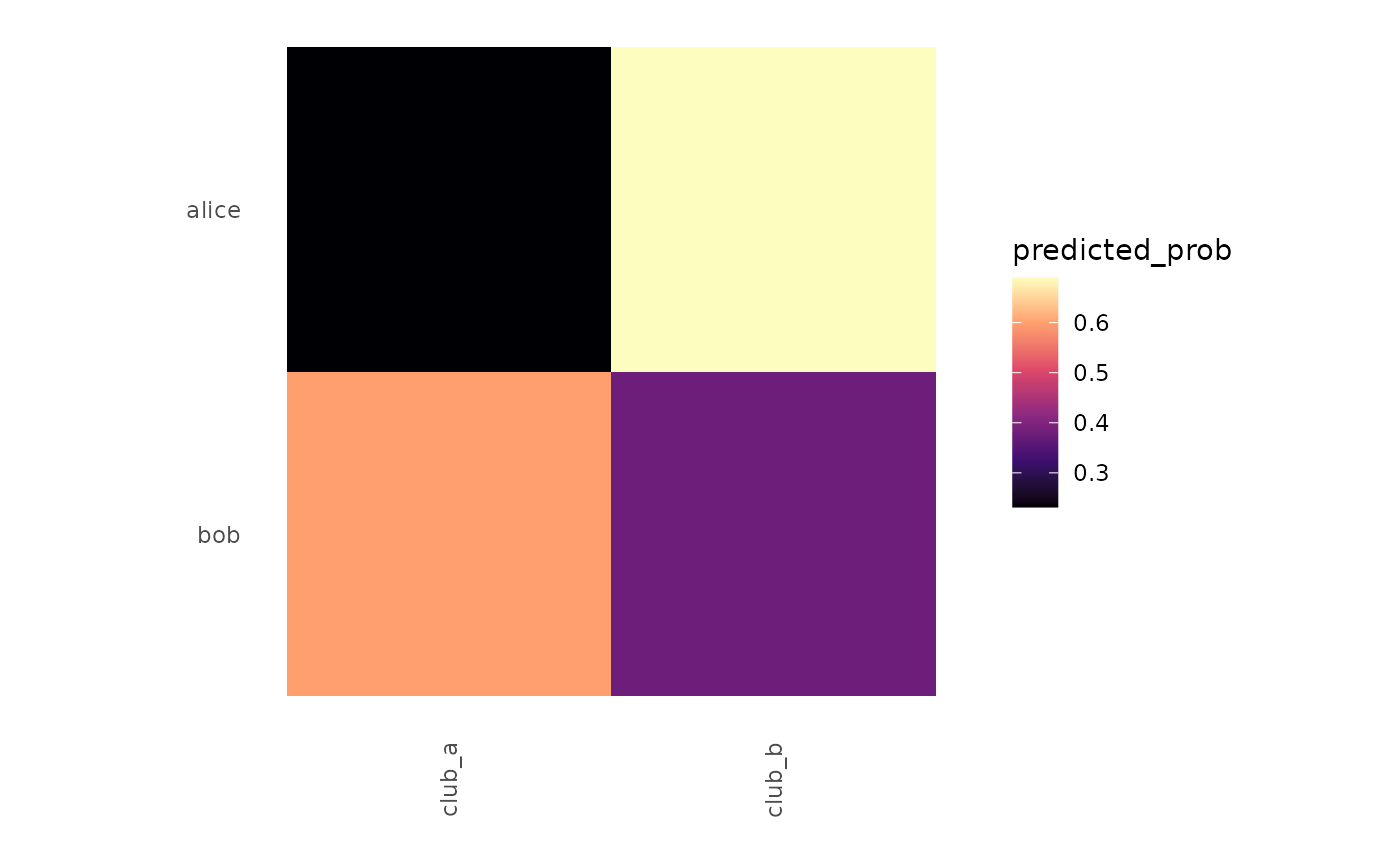
fitted_values <- matrix(
    c(-1.2, 0.4, 0.8, -0.5),
    nrow = 2,
    dimnames = list(c("alice", "bob"), c("club_a", "club_b"))
)

fit <- list(
    EZ = fitted_values,
    family = "binary",
    link = "logit",
    mode = "bipartite"
)

pred_net <- from_lame_fit(fit, value = "prob")
plot(pred_net, style = "heatmap")

# }