Impulse response analysis for network models

1 Overview

Impulse response functions (IRFs) measure how a shock to one part of the network propagates through the bilinear dynamics over time. Given the model $\Theta_t = A_t \Theta_{t-1} B_t' + M + \varepsilon_t$ , we inject a perturbation $S$ at time $t_0$ and track a network-level statistic over $H$ horizons:

$\Delta_0 = S, \quad \Delta_h = A_{t_0+h} \, \Delta_{h-1} \, B_{t_0+h}'$

At each horizon we compare a network statistic (density, degree, etc.) computed on the perturbed versus baseline network. The shock is applied once; subsequent horizons show how the estimated dynamics propagate it forward.

2 Fit a well-converged dynamic model

IRFs require a fitted model with time-varying $A$ and $B$ matrices. We use the Gaussian family for clean interpretation and simulate a 10-actor network with small innovation variances to keep the dynamics stable.

sim = simulate_dynamic_dbn(
  n = 10, p = 1, time = 15,
  sigma2 = 0.3, tauA2 = 0.03, tauB2 = 0.03,
  seed = 6886
)

fit = dbn(
  sim$Z,
  model   = "dynamic",
  family  = "gaussian",
  nscan   = 1000,
  burn    = 500,
  odens   = 2,
  verbose = FALSE
)

Always verify convergence before computing IRFs, since poorly converged chains produce unreliable credible intervals:

check_convergence(fit)
#>   sigma2   tau_A2   tau_B2       g2 
#> 319.5975 230.5858 180.6480 355.3089
#> 
#> Fraction in 1st window = 0.1
#> Fraction in 2nd window = 0.5 
#> 
#>  sigma2  tau_A2  tau_B2      g2 
#> -1.7963  0.8303 -2.2997 -1.1740

3 Building shock matrices

The build_shock() function creates structured perturbation matrices. Each type addresses a different counterfactual question.

m = 10

# shock a single directed edge (actor 1 -> actor 2)
S_edge = build_shock(m, type = "unit_edge", i = 1, j = 2, magnitude = 2)

# shock all outgoing edges from actor 1
S_node = build_shock(m, type = "node_out", i = 1, magnitude = 1)

# uniform shock to all edges
S_dens = build_shock(m, type = "density", magnitude = 0.5)

# custom block shock (e.g., a group-level perturbation)
S_custom = matrix(0, m, m)
S_custom[1:3, 4:6] = 1.0

4 Edge shock: effect on network density

How does shocking a single edge affect overall network connectivity? We add 2 units to the $(1,2)$ entry and track density (mean of off-diagonal entries) over 5 horizons.

irf_dens = compute_irf(
  fit,
  shock    = S_edge,
  H        = 5,
  t0       = 3,
  stat_fun = dbn::stat_density,
  n_draws  = 100
)

plot(irf_dens, title = "Edge Shock (1->2, +2) -> Network Density")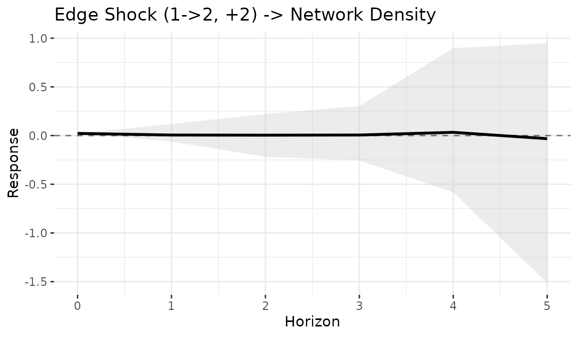

print(irf_dens)
#> Network Impulse Response Function
#> Model: dynamic 
#> Statistic: custom_function 
#> Shock time: 3 
#> 
#> Summary:
#>   horizon   mean median    sd   q025  q975    q10   q90
#> 1       0  0.022  0.022 0.000  0.022 0.022  0.022 0.022
#> 2       1  0.005 -0.002 0.046 -0.062 0.118 -0.042 0.062
#> 3       2  0.004  0.000 0.098 -0.219 0.222 -0.104 0.126
#> 4       3  0.006 -0.025 0.246 -0.255 0.303 -0.158 0.126
#> 5       4  0.033  0.021 0.341 -0.584 0.898 -0.303 0.285
#> 6       5 -0.032 -0.002 0.670 -1.512 0.948 -0.716 0.567

At horizon 0, the effect is exact: adding 2 to one off-diagonal cell in a 10-actor network changes density by $2 / (10 \times 9) \approx 0.022$ . At subsequent horizons, credible intervals widen as posterior uncertainty in the transition matrices compounds. The decay rate reflects the spectral properties of the estimated $A_t$ : eigenvalues near unity sustain the perturbation, while values well below unity produce rapid decay.

5 Node shock: effect on out-degree

What happens when an actor increases all outgoing ties at once? The node_out shock sets all entries in row $i$ (including the self-loop diagonal entry) to the specified magnitude.

irf_deg = compute_irf(
  fit,
  shock    = S_node,
  H        = 5,
  t0       = 3,
  stat_fun = function(X) stat_out_degree(X)[1],
  n_draws  = 100
)

plot(irf_deg, title = "Node-Out Shock (Actor 1, +1) -> Actor 1 Out-Degree")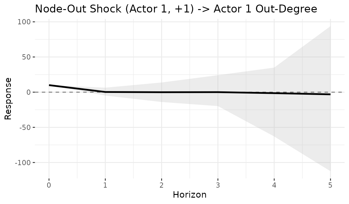

Actor 1’s out-degree jumps by 10 at horizon 0 (the shock sets all 10 entries in row 1, including the diagonal, to magnitude 1). The posterior mean of the effect decays toward zero at subsequent horizons, but the credible intervals widen substantially as posterior uncertainty in the transition matrices compounds across horizons. Wide credible intervals at longer horizons are typical and reflect how estimation uncertainty accumulates in multi-step propagation.

6 Edge shock: effect on reciprocity

Reciprocity is a nonlinear statistic (the correlation between $X_{ij}$ and $X_{ji}$ ). Unlike density, it depends on the baseline network structure, so there is posterior uncertainty even at horizon 0: the same shock produces different reciprocity changes depending on the baseline network, which varies across posterior draws.

irf_recip = compute_irf(
  fit,
  shock    = S_edge,
  H        = 5,
  t0       = 3,
  stat_fun = stat_reciprocity,
  n_draws  = 100
)

plot(irf_recip, title = "Edge Shock (1->2, +2) -> Network Reciprocity")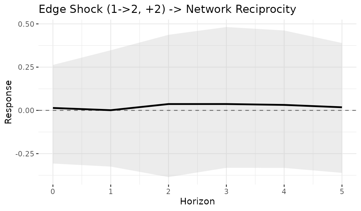

The nonzero credible interval at horizon 0 illustrates this distinction: for linear statistics like density, the horizon-0 effect is a deterministic function of the shock matrix, while for nonlinear statistics it interacts with the posterior distribution of the baseline network.

7 Comparing multiple shocks

Combining IRF results in a single figure allows side-by-side comparison across different shock types and statistics. Each panel uses its own y-axis scale because the statistics are on different scales.

irfs = list(
  "Edge -> Density"     = irf_dens,
  "Node -> Out-Degree"  = irf_deg,
  "Edge -> Recipr."     = irf_recip
)

df_all = do.call(rbind, lapply(names(irfs), function(nm) {
  d = irfs[[nm]]
  data.frame(
    horizon = d$horizon,
    mean    = d$mean,
    q025    = d$q025,
    q975    = d$q975,
    shock   = nm
  )
}))

ggplot(df_all, aes(x = horizon, y = mean)) +
  geom_ribbon(aes(ymin = q025, ymax = q975), alpha = 0.2) +
  geom_line(linewidth = 0.8) +
  geom_hline(yintercept = 0, linetype = "dashed") +
  facet_wrap(~ shock, scales = "free_y") +
  labs(x = "Horizon", y = "IRF", title = "Impulse Response Comparison") +
  theme_bw() +
  theme(
    panel.border = element_blank(),
    strip.background = element_rect(fill = "black", color = "black"),
    strip.text.x = element_text(color = "white", hjust = 0)
  )

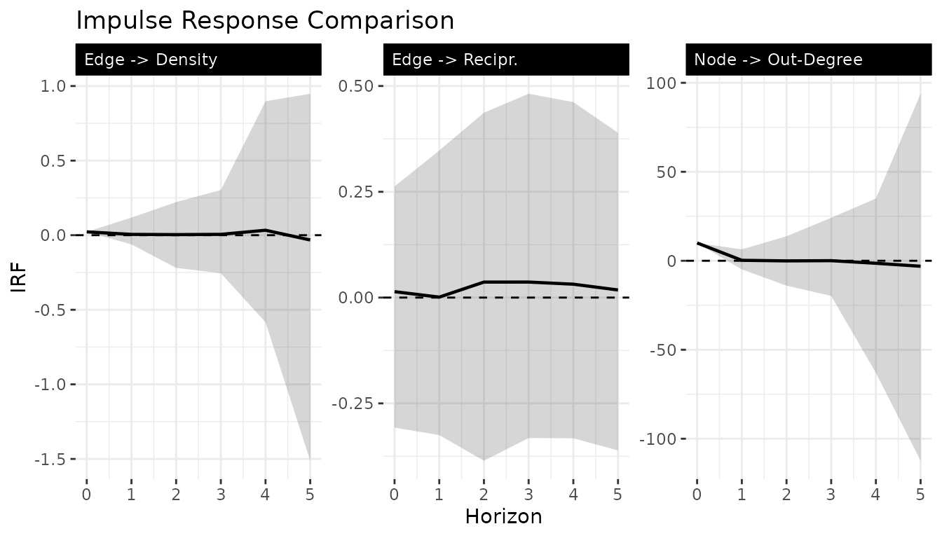
The key pattern to look for across all panels: a clear initial effect that decays toward zero, with credible intervals that widen but do not explode. An expanding credible interval that remains bounded is consistent with a well-identified model; explosive intervals suggest the estimated dynamics are unstable.

8 Interpreting IRFs

Horizon 0 captures the immediate, mechanical consequence of the shock. For linear statistics (density, degree), there is no posterior uncertainty at horizon 0 because the shock is a fixed constant. For nonlinear statistics (reciprocity, transitivity), there is uncertainty even at horizon 0 because the statistic interacts with the baseline network, which varies across posterior draws.

At horizons 1 and beyond, the estimated dynamics propagate the shock forward. Uncertainty widens because the transition matrices $A_t$ and $B_t$ are themselves estimated with posterior noise. The decay rate is governed by the spectral radius of $A$ : eigenvalues near unity sustain perturbations, while values well below unity produce rapid decay.

It is important to note that IRFs are counterfactual scenarios that assume the transition dynamics remain invariant to the shock. The credible intervals reflect posterior uncertainty in model parameters, not sampling variability in the observed data.

9 Available network statistics

The stat_fun argument accepts any function that maps a matrix to a scalar. Built-in statistics include stat_density() (mean of off-diagonal entries), stat_out_degree() and stat_in_degree() (row and column sums), stat_reciprocity() (correlation between $X_{ij}$ and $X_{ji}$ ), and stat_transitivity() (clustering coefficient). For degree-based statistics, wrap to extract a specific actor: function(X) stat_out_degree(X)[i].

10 Settings for publication

The examples above use moderate settings for vignette build times. For substantive analysis, increase both the model chain length and the number of IRF draws to ensure stable credible intervals:

fit = dbn(Y, model = "dynamic", family = "gaussian",
          nscan = 10000, burn = 5000, odens = 5)

irf = compute_irf(fit, shock = S, H = 10, t0 = 5,
                  stat_fun = dbn::stat_density, n_draws = 500)

11 Next steps

For a complete applied workflow with real data and IRFs, see vignette("applied_ir"). For piecewise models that compare pre- and post-regime influence structures, see vignette("piecewise_dbn").

Tosin Salau & Shahryar Minhas

2026-03-28