Piecewise-static models for structural change

1 Overview

Many political processes exhibit structural breaks, discrete moments when the rules governing network dynamics fundamentally change. The 2008 financial crisis reshuffled economic dependencies. The Arab Spring reorganized regional alliance patterns. A leadership transition can redirect a country’s foreign policy overnight.

The piecewise-static model handles this setting: you specify when breaks occurred and the model estimates how the influence structure differed across regimes. It fits block-constant influence matrices $A_k$ and $B_k$ for each regime $k = 1, \ldots, K$ :

$\Theta_t = A_{k(t)} \, \Theta_{t-1} \, B_{k(t)}^\top + M + \varepsilon_t$

The piecewise model sits between the static and dynamic extremes. It trades the time-point-level precision of the dynamic model for interpretability (each regime has a single, directly comparable influence matrix) and computational efficiency (estimating $K$ matrices instead of $T-1$ ).

Consideration	Piecewise	Dynamic
Breaks are discrete and known	X
Influence evolves smoothly		X
Comparing pre/post periods	X
Want interpretable regime summaries	X
Memory constraints (large networks)	X
Need time-point-specific estimates		X

2 Simulate data with a structural break

We simulate a network where the influence structure changes at a known break point, then check whether the model recovers the difference. The blocks argument specifies the ending time index of each block: block 1 covers $t = 1$ to 15, block 2 covers $t = 16$ to 30.

sim = simulate_piecewise_dbn(
  n      = 8,
  time   = 30,
  blocks = c(15, 30),
  p      = 1,
  sigma2 = 0.5,
  tau2   = 0.3,
  seed   = 6886
)

dim(sim$Y)
#> [1]  8  8  1 30

# block structure
sim$block_info$K
#> [1] 2
sim$block_info$boundaries
#> [1]  0 15 30
sim$block_info$lengths
#> [1] 15 15

# average element-wise difference between regime A matrices
round(mean(abs(sim$true_A[[1]] - sim$true_A[[2]])), 3)
#> [1] 0.135

The element-wise difference between the two true $A$ matrices confirms that the data-generating process produces genuinely different regimes.

3 Fit the piecewise model

Pass the known break points via blocks. The model estimates separate $A_k$ and $B_k$ for each regime while sharing the baseline mean $M$ .

fit = dbn(
  sim$Y,
  model   = "piecewise",
  family  = "ordinal",
  blocks  = c(15, 30),
  nscan   = 1000,
  burn    = 500,
  odens   = 2,
  verbose = FALSE
)

summary(fit)
#> Piecewise-Static DBN Model Summary
#> ========================================
#> 
#> Data:
#>   Nodes: 8
#>   Relations: 1
#>   Time points: 30
#> 
#> Block Structure:
#>   Number of blocks: 2
#>   Boundaries: 0 -> 15 -> 30
#>   Block lengths: 15, 15
#> 
#> MCMC:
#>   Iterations: 1000
#>   Burn-in: 500
#>   Saved draws: 500
#> 
#> Parameter Estimates (posterior mean [95% CI]):
#>   s2: 1 [1, 1]
#>   t2: 0.0287 [0.0216, 0.0381]
#>   g2: 0.0721 [0.0451, 0.1178]
#> 
#> Block-Specific Influence (||A_k||_F):
#>   block_1: 1.278 [1.018, 1.555]
#>   block_2: 1.283 [1.019, 1.581]

4 Convergence diagnostics

check_convergence(fit)
#>       t2       g2 
#> 197.9471 337.1320
#> 
#> Fraction in 1st window = 0.1
#> Fraction in 2nd window = 0.5 
#> 
#>      t2      g2 
#> -1.4387  0.3922
plot_trace(fit, pars = c("s2", "t2", "g2"))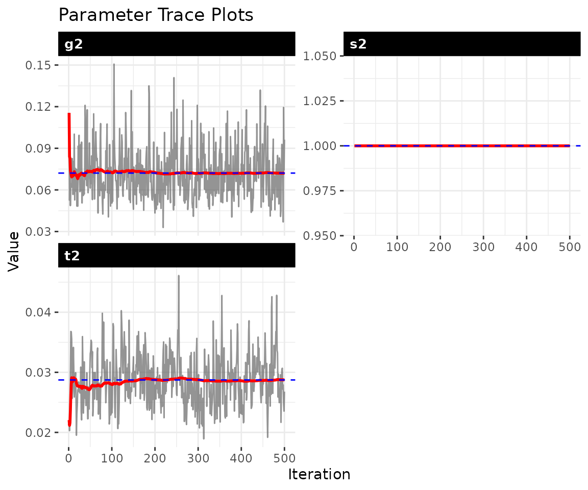

5 Regime comparison

The compare_blocks() function quantifies differences between regimes with posterior uncertainty. The output reports the posterior mean of the Frobenius norm $\|A_k - A_{k+1}\|$ , a 95% credible interval, and the posterior probability that the difference exceeds a substantively meaningful threshold (default 0.1). A high probability indicates strong evidence that the influence structure genuinely changed, not just sampling noise.

regime_diffs = compare_blocks(fit)

6 Extracting regime-specific influence

Each regime has its own estimated $A$ and $B$ matrices stored in the fit object.

A1_est = fit$A_blocks[[1]]
A2_est = fit$A_blocks[[2]]

The compare_blocks() result is the primary tool for assessing whether the influence structure genuinely changed between regimes. For entry-level comparisons of individual $A$ elements, use a larger network ( $n \geq 20$ ).

7 Visualizing influence change

The difference $A_2 - A_1$ shows which sender-influence relationships changed most across regimes. Red entries indicate actors whose influence increased in regime 2; blue entries indicate decreased influence.

diff_A = A2_est - A1_est
n = nrow(diff_A)

df_heatmap = expand.grid(
  receiver = seq_len(n),
  sender   = seq_len(n)
)
df_heatmap$value = as.vector(diff_A)

ggplot(df_heatmap, aes(x = sender, y = receiver, fill = value)) +
  geom_tile() +
  scale_fill_gradient2(
    low = "blue", mid = "white", high = "red",
    name = expression(Delta * A)
  ) +
  labs(
    title = "Change in Sender Influence: Regime 2 vs. Regime 1",
    x = "Sender (Influenced By)", y = "Sender (Influences)"
  ) +
  coord_equal() +
  theme_bw() +
  theme(panel.border = element_blank())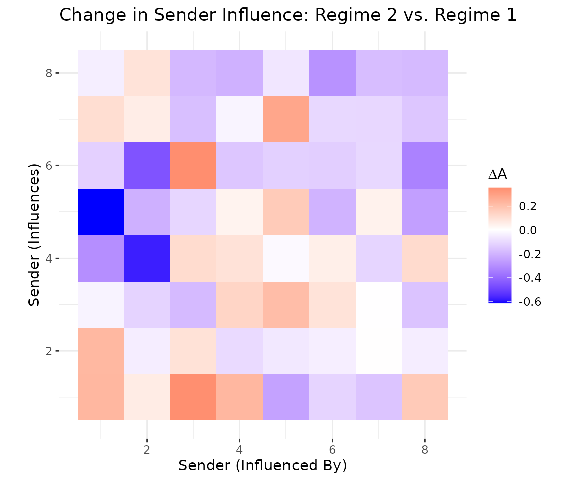

8 Speed and memory advantages

The piecewise model estimates $K$ influence matrices instead of $T-1$ , pooling data within each regime. This makes it faster and more memory-efficient than the dynamic model, particularly for longer time series.

sim_t = simulate_piecewise_dbn(n = 10, time = 30, blocks = 3, seed = 6886)

t_pw = system.time({
  fit_pw = dbn(sim_t$Y, model = "piecewise", blocks = 3,
               nscan = 1000, burn = 500, verbose = FALSE)
})

t_dyn = system.time({
  fit_dyn = dbn(sim_t$Y, model = "dynamic",
                nscan = 1000, burn = 500, verbose = FALSE)
})

data.frame(
  model   = c("Piecewise", "Dynamic"),
  seconds = round(c(t_pw["elapsed"], t_dyn["elapsed"]), 1)
)
#>       model seconds
#> 1 Piecewise     2.0
#> 2   Dynamic    13.1

For large networks, use store_theta = FALSE to avoid storing the full $\Theta$ posterior (which scales as $n^2 \times T \times \text{draws}$ ). This retains $A$ , $B$ , $M$ , variance posteriors, convergence diagnostics, and compare_blocks() support while substantially reducing memory.

fit_full = dbn(sim$Y, model = "piecewise", blocks = c(15, 30),
               nscan = 200, burn = 100, verbose = FALSE, store_theta = TRUE)
fit_lean = dbn(sim$Y, model = "piecewise", blocks = c(15, 30),
               nscan = 200, burn = 100, verbose = FALSE, store_theta = FALSE)

data.frame(
  storage = c("With Theta", "Without Theta"),
  mb      = round(c(object.size(fit_full), object.size(fit_lean)) / 1e6, 2)
)
#>         storage   mb
#> 1    With Theta 3.96
#> 2 Without Theta 0.84

9 Specifying blocks

The blocks argument is flexible. A single integer creates that many equal-sized blocks. A vector of integers specifies the ending time index of each block. Named vectors improve readability for applied work.

# integer: equal-sized regimes
fit = dbn(Y, model = "piecewise", blocks = 4)

# vector of endpoints
fit = dbn(Y, model = "piecewise", blocks = c(10, 25, 40))

# named vector for interpretability
fit = dbn(Y, model = "piecewise",
          blocks = c(pre_war = 15, war = 30, post_war = 45))

10 Gaussian family

The piecewise model supports all three outcome families. For continuous data, switch to family = "gaussian":

fit_gauss = dbn(
  sim$Y_continuous,
  model   = "piecewise",
  family  = "gaussian",
  blocks  = c(15, 30),
  nscan   = 1000,
  burn    = 500,
  odens   = 2,
  verbose = FALSE
)

summary(fit_gauss)
#> Piecewise-Static DBN Model Summary
#> ========================================
#> 
#> Data:
#>   Nodes: 8
#>   Relations: 1
#>   Time points: 30
#> 
#> Block Structure:
#>   Number of blocks: 2
#>   Boundaries: 0 -> 15 -> 30
#>   Block lengths: 15, 15
#> 
#> MCMC:
#>   Iterations: 1000
#>   Burn-in: 500
#>   Saved draws: 500
#> 
#> Parameter Estimates (posterior mean [95% CI]):
#>   s2: 0.9781 [0.8938, 1.0614]
#>   t2: 0.0202 [0.015, 0.027]
#>   g2: 0.0947 [0.0602, 0.1438]
#> 
#> Block-Specific Influence (||A_k||_F):
#>   block_1: 1.785 [1.322, 2.47]
#>   block_2: 1.828 [1.377, 2.475]

11 Applied example: UNGA voting and the 2008 financial crisis

This example examines UN General Assembly voting alignment using the financial crisis as a structural break. It requires the peacesciencer package. Because it uses external data, we show the code and pre-computed output rather than evaluating inline.

library(peacesciencer)

# build dyadic panel 1995-2015
dyads = create_dyadyears(subset_years = 1995:2015) |>
  add_fpsim()

# select ~100 countries with complete data
years = 1995:2015
complete_countries = Reduce(intersect, lapply(years, function(y) {
  unique(c(dyads$ccode1[dyads$year == y], dyads$ccode2[dyads$year == y]))
}))

country_coverage = table(c(
  dyads$ccode1[dyads$ccode1 %in% complete_countries],
  dyads$ccode2[dyads$ccode2 %in% complete_countries]
))
top_countries = as.numeric(
  names(sort(country_coverage, decreasing = TRUE))[1:100]
)

# build [n, n, 1, T] array of kappavv similarity scores
dyads_sub = dyads[dyads$ccode1 %in% top_countries &
                    dyads$ccode2 %in% top_countries, ]
actor_codes = sort(unique(c(dyads_sub$ccode1, dyads_sub$ccode2)))
n_actors = length(actor_codes)
code_to_idx = setNames(seq_along(actor_codes), actor_codes)

Y_unga = array(NA_real_, dim = c(n_actors, n_actors, 1, length(years)))
for (i in seq_len(nrow(dyads_sub))) {
  row_i = code_to_idx[as.character(dyads_sub$ccode1[i])]
  col_j = code_to_idx[as.character(dyads_sub$ccode2[i])]
  t_idx = which(years == dyads_sub$year[i])
  Y_unga[row_i, col_j, 1, t_idx] = dyads_sub$kappavv[i]
}
for (t in seq_along(years)) diag(Y_unga[, , 1, t]) = NA

# fit piecewise model with 2008 crisis as break point
t_break = which(years == 2008)
fit_crisis = dbn(
  Y_unga,
  model  = "piecewise",
  family = "gaussian",
  blocks = c(t_break, length(years)),
  nscan  = 5000,
  burn   = 2000,
  odens  = 5,
  store_theta = FALSE,
  verbose = TRUE
)

# did the influence structure change?
compare_blocks(fit_crisis)
#> Block Comparison Results (A)
#> block_1 vs block_2: ||dA|| = 2.34 [1.89, 2.91]
#>   P(||dA|| > 0.1) = 1

# which actors' influence changed most?
A_pre  = fit_crisis$A_blocks[[1]]
A_post = fit_crisis$A_blocks[[2]]
influence_change = rowSums(abs(A_post)) - rowSums(abs(A_pre))

A high probability that the Frobenius norm exceeds the threshold indicates the crisis genuinely altered alignment dynamics. In typical applications, emerging market countries from Latin America, Asia, and Africa show increased influence on alignment patterns post-2008, while G7 nations show flat or declining dynamic influence. Countries that actively built coalitions (Brazil, Turkey, South Africa) tend to emerge as gainers. Substantive conclusions require longer MCMC runs, robustness checks with alternative break points, and domain expertise.

12 Scaling to large networks

Actors	Theta Storage	Expected Runtime	Memory
50	OK	1-5 min	< 1 GB
100	Marginal	5-20 min	2-8 GB
200	Disable	30-90 min	1-4 GB
500+	Disable	Hours	5-20 GB

For 200+ actors, always use store_theta = FALSE. You retain $A$ , $B$ , $M$ , variance posteriors, convergence diagnostics, and compare_blocks() support; you lose full $\Theta$ posterior uncertainty.

fit_large = dbn(
  Y_large,
  model       = "piecewise",
  family      = "gaussian",
  blocks      = c(25, 50),
  store_theta = FALSE,
  nscan       = 5000,
  burn        = 2000,
  odens       = 5,
  verbose     = TRUE
)

13 Practical guidance

Choosing break points

Good candidates include known events (war onset, treaty signing), policy interventions (sanctions, trade agreements), and external shocks (financial crises, pandemics). If uncertain about break point location, fit multiple models with different break specifications and compare with compare_dbn().

How many regimes?

Time Points	Max Regimes
20-30	2-3
30-50	3-4
50-100	4-6

Relationship to other models

Piecewise with $K = 1$ is equivalent to the static model. Compared to the dynamic model, piecewise trades time-point precision for interpretability and speed. Compared to the HMM model, piecewise requires the analyst to specify break points rather than discovering them from the data.

14 Next steps

For smoothly evolving dynamics, see vignette("dynamic_dbn"). For data-driven regime discovery, see vignette("hmm_dbn"). For impulse response analysis, see vignette("impulse_response"). For a complete applied workflow with IRFs, see vignette("applied_ir").

Shahryar Minhas

2026-03-29