Regime-switching (HMM) bilinear network models

1 Overview

The HMM variant of the dynamic bilinear network model allows for regime-switching dynamics. At each time point, the network is governed by one of $R$ discrete regimes, each with its own influence matrices $A_r$ and $B_r$ . Transitions between regimes follow a Markov chain with an estimated transition matrix $\Pi$ :

$\Theta_t = A_{s_t} \, \Theta_{t-1} \, B_{s_t}^\top + M + \varepsilon_t, \quad s_t \sim \text{Markov}(\Pi)$

This model is appropriate when network dynamics exhibit abrupt structural breaks and the analyst wants the model to discover when those breaks occur, rather than specifying them in advance. For known break points, the piecewise model provides more stable inference with fewer parameters (see vignette("piecewise_dbn")).

Regime identification improves with network size, time series length, and the magnitude of the structural difference between regimes. For small networks ( $n < 15$ ) or subtle regime changes, the piecewise model with known break points is a more reliable choice.

2 Simulate a regime-switching network

We simulate a two-regime network with 12 actors over 30 time periods. The high transition_prob (0.9) means each regime persists for several consecutive periods before switching. The large tau_A2 and tau_B2 values (0.8) create regimes with substantially different dynamics, which is important for reliable regime identification.

sim = simulate_hmm_dbn(
  n     = 12,
  p     = 1,
  time  = 30,
  R     = 2,
  sigma2        = 0.3,
  tau_A2        = 0.8,
  tau_B2        = 0.8,
  transition_prob = 0.9,
  seed  = 6886
)

dim(sim$Y)
#> [1] 12 12  1 30

# true regime sequence and frequencies
sim$S
#>  [1] 2 2 2 2 2 2 2 2 2 1 2 2 2 2 2 2 2 2 2 1 1 1 1 1 1 1 1 1 1 1
table(sim$S)
#> 
#>  1  2 
#> 12 18

The true regime labels show which regime generated each time point. With two regimes and a transition probability of 0.9, we expect each regime to persist for an average of 10 consecutive periods before switching.

3 Fit the HMM model

We set model = "hmm" and specify R = 2 regimes. The sampler jointly estimates regime-specific dynamics matrices ( $A_r$ , $B_r$ ), the transition matrix $\Pi$ , and the regime labels $s_t$ .

fit = dbn(
  sim$Y,
  model   = "hmm",
  family  = "ordinal",
  R       = 2,
  nscan   = 1000,
  burn    = 500,
  odens   = 2,
  verbose = FALSE
)

4 Model summary and transition matrix

The summary reports the posterior mean transition matrix $\Pi$ and variance parameters. The diagonal of $\Pi$ indicates regime persistence: values near 1 mean regimes tend to stick, while large off-diagonal values indicate frequent switching.

summary(fit)
#> Regime-switching (HMM) DBN model
#>   nodes     : 12 
#>   relations : 1 
#>   time pts  : 30 
#>   regimes   : 2 
#> 
#>        mean  2.5%  97.5%
#> sigma2 1.000 1.000 1.000
#> tau_A2 0.041 0.037 0.046
#> tau_B2 0.039 0.035 0.043
#> g2     0.030 0.025 0.034
#> 
#> Posterior mean transition matrix Pi:
#>       [,1]  [,2]
#> [1,] 0.691 0.309
#> [2,] 0.504 0.496

Two things to note about the estimated $\Pi$ . First, the model’s regime labels may not match the simulation’s — this is the standard label-switching issue in mixture models and does not affect the substantive results. Second, with the moderate chain length used here (nscan = 1000), the transition matrix has substantial posterior uncertainty. Recovering the true persistence (0.9 on the diagonal) requires longer chains and larger networks; with $n = 12$ actors and 30 time points, the model has limited data per regime to pin down $\Pi$ precisely. For substantive work, run at least nscan = 5000 with burn = 2000.

5 Regime probabilities

The posterior probability of each regime at each time point provides the model’s classification of the time series into regimes. Probabilities near 0 or 1 indicate confident classification; values near 0.5 indicate ambiguity. Regime identification depends on how different the regimes are (controlled by tau_A2 and tau_B2 in the simulation) and how much data is available per time point (number of actors).

plot_regime_probs(fit)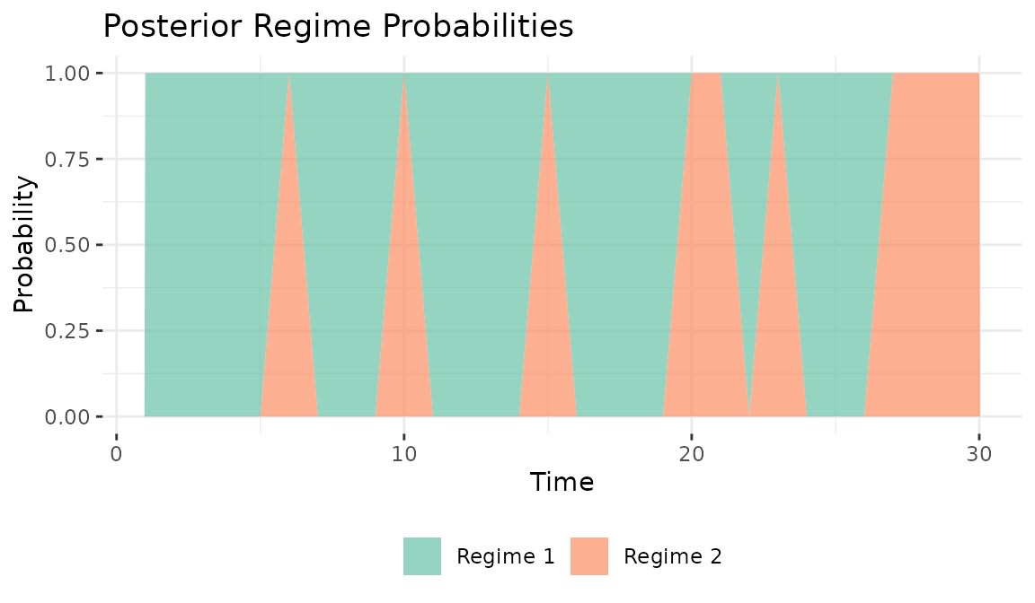

The regime_probs() function returns the underlying probability matrix for custom analysis. Each row sums to 1 across regimes.

probs = regime_probs(fit)
head(probs, 10)
#>        Regime1 Regime2
#> Time1        1       0
#> Time2        1       0
#> Time3        1       0
#> Time4        1       0
#> Time5        1       0
#> Time6        0       1
#> Time7        1       0
#> Time8        1       0
#> Time9        1       0
#> Time10       0       1

6 Model diagnostics

The default plot() method for HMM fits provides a combined diagnostic view: regime probabilities, the estimated transition matrix, and MCMC trace plots for monitoring convergence.

plot(fit)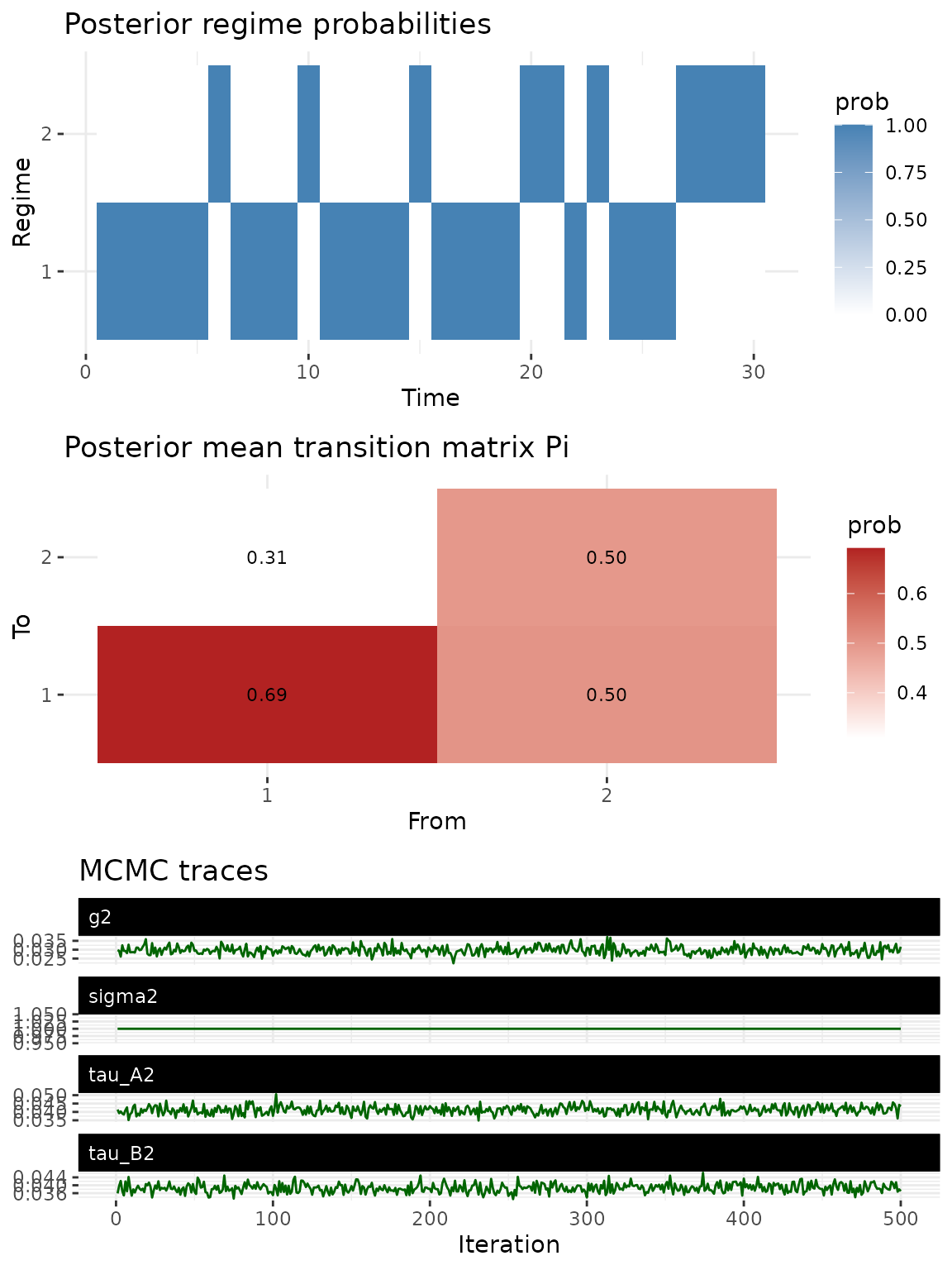

7 Dyad trajectory

The dyad_path() function tracks a specific bilateral relationship over time with posterior credible intervals, averaging across regime assignments.

dyad_path(fit, i = 2, j = 5)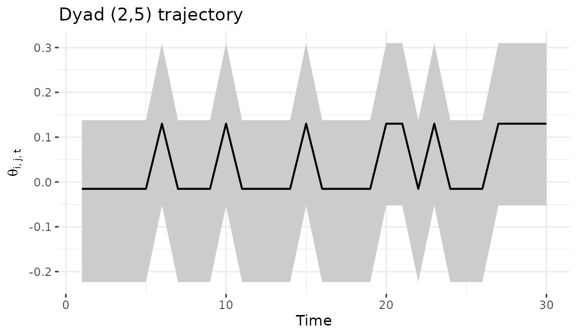

8 Forecasting

The predict() method samples future regime states from $\Pi$ and propagates the regime-specific bilinear dynamics forward. This means forecast uncertainty reflects both posterior uncertainty in $A_r$ and $B_r$ and uncertainty about which regime will be active in future periods.

pred = predict(fit, H = 5, draws = 100, summary = "mean")
dim(pred)
#> [1] 12 12  1  5

9 When to use HMM

The HMM model is appropriate when network dynamics exhibit discrete structural breaks (such as policy changes, crises, or regime transitions) and the analyst wants data-driven discovery of when those breaks occur. The number of regimes $R$ should be small (2-5), and the network should have enough actors and time points to identify regime structure. For smoothly evolving dynamics without discrete breaks, model = "dynamic" is a better choice. For known break points, model = "piecewise" provides more stable inference. For large networks (50+ actors), model = "lowrank" offers better scalability.

Tosin Salau & Shahryar Minhas

2026-03-28