Dynamic bilinear network models

1 The model

The dynamic bilinear model allows the influence matrices $A_t$ and $B_t$ to change over time, capturing settings where the rules governing network evolution are themselves evolving:

$\Theta_t = A_t \, \Theta_{t-1} \, B_t^\top + M + \varepsilon_t$

Entry $a_{i,i',t}$ of the sender influence matrix $A_t$ measures how strongly actor $i'$ ’s past sending behavior predicts actor $i$ ’s current sending at time $t$ . The receiver matrix $B_t$ captures the analogous pattern on the targeting side. The baseline mean $M$ absorbs stable dyad-specific tendencies that persist regardless of the dynamics.

Two additional parameters govern how rapidly the influence structure reorganizes. The innovation variances $\tau_A^2$ and $\tau_B^2$ control step-to-step variation in $A_t$ and $B_t$ : values near zero indicate a nearly static structure, while larger values allow rapid reorganization. When ar1 = TRUE, the model adds persistence parameters $\rho_A$ and $\rho_B$ that measure mean reversion. Values of $\rho$ near 1 indicate that the influence structure is highly persistent; values near 0 indicate rapid reversion to the prior mean.

2 Simulate data

We generate a Gaussian network with time-varying influence matrices. Setting ar1 = TRUE gives the influence matrices AR(1) dynamics, so each period’s influence structure is a noisy version of the previous period’s rather than an uncorrelated random walk. The high persistence ( $\rho = 0.9$ ) and small innovation variance ( $\tau^2 = 0.04$ ) create smoothly evolving dynamics that are easier to recover from limited data.

sim = simulate_dynamic_dbn(
  n      = 8,
  p      = 1,
  time   = 15,
  sigma2 = 0.3,
  tauA2  = 0.04,
  tauB2  = 0.04,
  ar1    = TRUE,
  rhoA   = 0.9,
  rhoB   = 0.9,
  seed   = 6886
)

Y = sim$Z
dim(Y)
#> [1]  8  8  1 15

3 Fit the model

We set ar1 = TRUE so the model uses AR(1) dynamics for $A_t$ and $B_t$ , and update_rho = TRUE so the persistence parameters are estimated from the data rather than fixed at a default value.

fit = dbn(
  Y,
  family     = "gaussian",
  model      = "dynamic",
  nscan      = 1000,
  burn       = 500,
  odens      = 2,
  ar1        = TRUE,
  update_rho = TRUE,
  verbose    = FALSE
)

4 Convergence diagnostics

The trace plots should show stationary chains with no drift. For the dynamic model, the key parameters are $\sigma^2$ (process noise), $\tau_A^2$ and $\tau_B^2$ (innovation variances), and $\rho_A$ and $\rho_B$ (persistence).

check_convergence(fit)
#>    sigma2    tau_A2    tau_B2        g2 
#> 498.11527  77.69979  65.80980 392.33129
#> 
#> Fraction in 1st window = 0.1
#> Fraction in 2nd window = 0.5 
#> 
#>  sigma2  tau_A2  tau_B2      g2 
#> -2.1739  0.5757 -1.2306 -0.6350

plot_trace(fit, pars = c("sigma2", "tau_A2", "tau_B2", "rho_A", "rho_B"))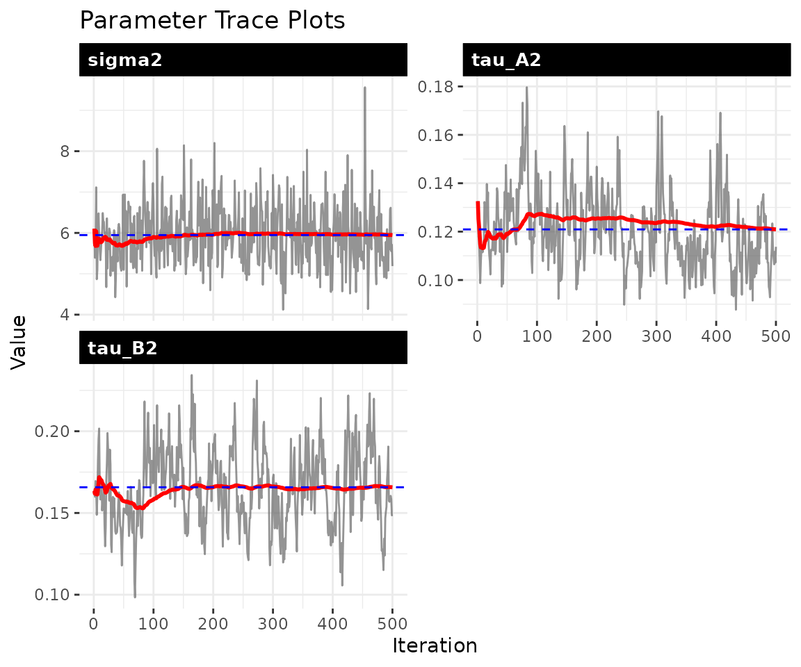

5 Parameter recovery

Scalar parameters

param_summary(fit)
#>    parameter       mean         sd       q2.5       q50     q97.5
#> 1     sigma2 5.94737738 0.72658796 4.70775216 5.9317598 7.4606929
#> 2     tau_A2 0.12091809 0.01561779 0.09610393 0.1194444 0.1556927
#> 3     tau_B2 0.16572224 0.02368038 0.12372206 0.1642472 0.2142344
#> 4         g2 0.09200445 0.02070456 0.05860016 0.0891350 0.1392518
#> 5       rhoA 0.78392539 0.03691866 0.70602944 0.7861769 0.8479822
#> 6       rhoB 0.74915741 0.04180474 0.66540326 0.7519273 0.8301224
#> 7 sigma2_obs 0.91885799 0.05993262 0.80695241 0.9171687 1.0322075

The model estimates variance parameters that govern the dynamics. The internal parameterization may differ in scale from the simulation inputs, so direct comparison of scalar values is not always meaningful. The most informative validation is whether the model recovers the latent network trajectories.

Latent network recovery

The model’s primary output is the latent network state $\Theta_t$ . We compare the posterior mean of $\Theta_t + M$ to the true values across all dyads and time points. Strong correlation along the diagonal indicates that the model is capturing both the cross-sectional structure and the temporal dynamics.

Theta_mean = apply(fit$Theta, 1:4, mean)
M_mean = apply(fit$M, 1:3, mean)

n_act = dim(sim$Theta)[1]
Tt = dim(sim$Theta)[4]

true_vals = numeric(0)
est_vals  = numeric(0)

for (t in seq_len(Tt)) {
  true_mat = sim$Theta[, , 1, t]
  est_mat  = Theta_mean[, , 1, t] + M_mean[, , 1]
  mask = !is.na(true_mat)
  true_vals = c(true_vals, true_mat[mask])
  est_vals  = c(est_vals, est_mat[mask])
}

df_theta = data.frame(truth = true_vals, estimate = est_vals)
r_sq = round(cor(df_theta$truth, df_theta$estimate)^2, 3)

ggplot(df_theta, aes(x = truth, y = estimate)) +
  geom_abline(slope = 1, intercept = 0, linetype = "dashed") +
  geom_point(alpha = 0.1, size = 0.8) +
  labs(
    title    = "Recovery of Latent Network State",
    subtitle = paste0("R-Squared = ", r_sq, " (All Dyads x Time Points)"),
    x = expression("True " * Theta[t]),
    y = expression("Posterior Mean " * Theta[t] + M)
  ) +
  theme_bw() +
  theme(panel.border = element_blank())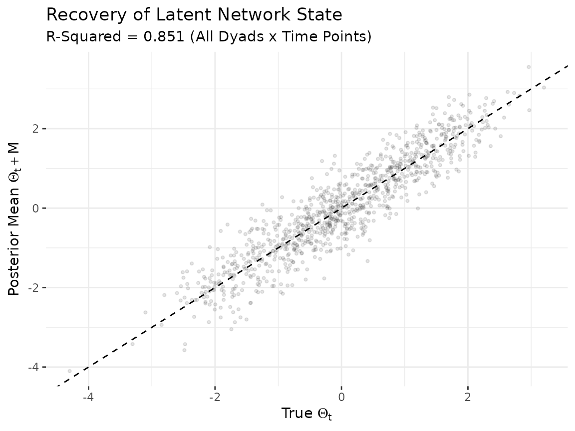

Each point represents one off-diagonal dyad at one time point. Some scatter is expected due to posterior shrinkage and estimation uncertainty, but the bulk of points should cluster along the diagonal.

6 Dyad trajectories

The dyad_path() function tracks how a specific bilateral relationship evolves over time, with a ribbon showing the posterior credible interval. Wider ribbons indicate greater uncertainty about the trajectory of that particular relationship.

dyad_path(fit, i = 1, j = 2)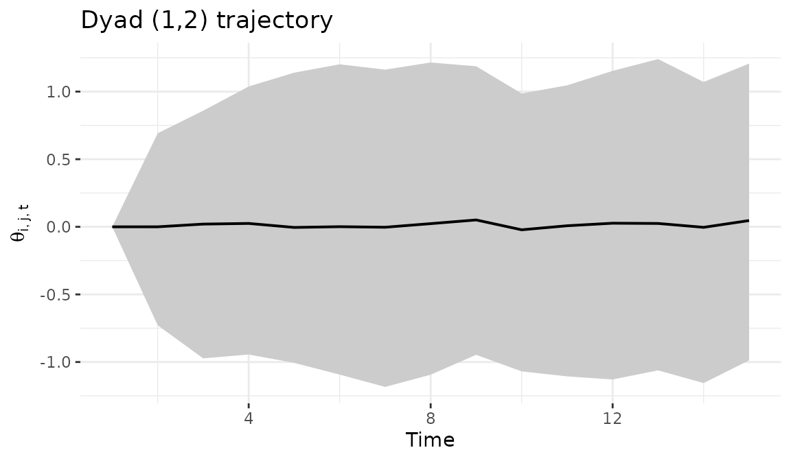

7 Forecasting

We generate forecasts 5 steps ahead by propagating the estimated dynamics forward. Each of the 200 posterior draws produces a different forecast trajectory (reflecting uncertainty in $A$ , $B$ , and $\sigma^2$ ), and summary = "mean" averages across them.

fc = predict(fit, H = 5, S = 200, summary = "mean")
dim(fc)
#> [1] 8 8 1 5

The resulting array has dimensions [actors, actors, relations, horizon]. These forecasts assume the final-period dynamics continue unchanged, so they are most informative over short horizons.

8 Network statistics over time

The network_summary() function tracks a network-level statistic across time with posterior credible intervals, providing a macro-level view of how the network evolves.

ns = network_summary(fit, stat = "density")
head(ns)
#>   time      mean     lower     upper
#> 1    1 0.4633571 0.3750000 0.5535714
#> 2    2 0.4594286 0.3928571 0.5357143
#> 3    3 0.4991071 0.4285714 0.5714286
#> 4    4 0.4861786 0.4107143 0.5714286
#> 5    5 0.4926786 0.4107143 0.5714286
#> 6    6 0.4603929 0.3750000 0.5357143

The edge_prob() function computes the posterior probability that each edge is positive at a given time point. Values near 1 indicate reliably positive edges; values near 0.5 indicate substantial uncertainty about the sign.

ep = edge_prob(fit, rel = 1, time = dim(Y)[4])
round(ep[1:5, 1:5], 2)
#>      [,1] [,2] [,3] [,4] [,5]
#> [1,]   NA 0.99 0.83 0.75 0.72
#> [2,] 0.53   NA 0.38 0.23 0.80
#> [3,] 0.36 0.25   NA 0.14 0.06
#> [4,] 0.04 0.40 0.27   NA 0.92
#> [5,] 0.51 0.86 0.96 0.22   NA

9 Bipartite networks

The package automatically detects bipartite networks when the sender and receiver dimensions differ. Passing a rectangular array causes the model to estimate $A$ as n_row x n_row (sender dynamics) and $B$ as n_col x n_col (receiver dynamics).

sim_bp = simulate_dynamic_dbn(
  n = 8, n_col = 6, p = 1, time = 12, seed = 6886
)

fit_bp = dbn(
  sim_bp$Z,
  model   = "dynamic",
  family  = "gaussian",
  nscan   = 1000,
  burn    = 500,
  odens   = 2,
  verbose = FALSE
)
summary(fit_bp)

10 Parallel computation

The dynamic model parallelizes row-wise FFBS updates via OpenMP. For networks with 15 or more actors, multi-threading produces meaningful speedups (typically 2-4x with 4-8 cores).

set_dbn_threads(parallel::detectCores(logical = FALSE))

11 Scaling guidance

For larger networks, the main constraint is RAM. Use estimate_memory() before fitting, and adjust time_thin and odens to manage memory.

estimate_memory(
  n_row = 50, n_col = 50, p = 1, Tt = 30,
  nscan = 1000, burn = 500, odens = 2,
  time_thin = 2, family = "gaussian"
)
#> Dynamic DBN memory estimate:
#>   Network:   50 x 50, 1 relation(s), 30 time points
#>   MCMC:      500 draws (nscan=1000, odens=2)
#>   Time thin: 2 (keeping 15 of 30 time points)
#>   --------------------------------
#>   Theta:    0.14 GB
#>   A:        0.14 GB
#>   B:        0.14 GB
#>   M:        0.01 GB
#>   --------------------------------
#>   TOTAL:    0.43 GB

For 100+ actors, expect to need 16-32 GB depending on settings. Increasing time_thin and odens are the most effective ways to reduce memory usage.

12 Next steps

For impulse response analysis that traces how shocks propagate through the estimated dynamics, see vignette("impulse_response"). For models with known structural breaks where the influence structure shifts at discrete time points, see vignette("piecewise_dbn"). For large networks (50+ actors), see vignette("lowrank_dbn").

Tosin Salau & Shahryar Minhas

2026-03-28