Low-rank bilinear network models

1 Overview

The low-rank model factorizes the sender dynamics matrix as:

$A_t = U \, \text{diag}(\alpha_t) \, U^\top$

where $U$ is an $n \times r$ orthogonal matrix (constrained to the Stiefel manifold) and $\alpha_t$ is a vector of time-varying factor strengths. This reduces the number of free parameters from $n^2$ to $n \times r + r$ . For a 50-actor network, the full dynamic model requires estimating 2,500 entries per time point, while a rank-3 low-rank model requires only 153 ( $50 \times 3 + 3$ ).

The columns of $U$ define latent groups of actors that share similar influence patterns. The factor trajectories $\alpha_t$ capture how strongly each latent dimension drives the dynamics at each time point. This structure makes the model tractable for larger networks where the full dynamic model becomes prohibitively expensive.

2 When to use low-rank

The low-rank model is designed for networks with 50 or more actors where the full dynamic model is computationally prohibitive. The parameter savings grow quadratically with network size:

Network Size	Full Dynamic Parameters	Rank-3 Low-Rank Parameters
20 actors	400	63
50 actors	2,500	153
100 actors	10,000	303

For smaller networks where full flexibility is affordable, use model = "dynamic". For known structural break points, use model = "piecewise".

3 Memory estimation

Before fitting, check RAM requirements with estimate_memory(). This is particularly important for the low-rank model because its primary use case is larger networks where memory is the binding constraint.

estimate_memory(
  n_row = 50, n_col = 50, p = 1, Tt = 30,
  nscan = 5000, burn = 2000, odens = 5,
  family = "ordinal"
)
#> Dynamic DBN memory estimate:
#>   Network:   50 x 50, 1 relation(s), 30 time points
#>   MCMC:      1000 draws (nscan=5000, odens=5)
#>   Time thin: 1 (keeping 30 of 30 time points)
#>   --------------------------------
#>   Theta:    0.56 GB
#>   Z:        0.56 GB
#>   A:        0.56 GB
#>   B:        0.56 GB
#>   M:        0.02 GB
#>   --------------------------------
#>   TOTAL:    2.25 GB

4 Simulate data

We simulate a 10-node network with rank $r = 2$ , meaning the sender dynamics are driven by two latent factors. We use the Gaussian family (sim$Z) for this demonstration because it provides sharper factor identification than the ordinal family at small network sizes. The model’s primary use case is networks with 50+ actors where the ordinal family works well; this small example illustrates the API and factor trajectory interpretation.

sim = simulate_lowrank_dbn(
  n          = 10,
  p          = 1,
  time       = 15,
  r          = 2,
  sigma2     = 0.3,
  tau_alpha2 = 0.1,
  tauB2      = 0.04,
  seed       = 6886
)

dim(sim$Z)
#> [1] 10 10  1 15

5 Fit the model

The key argument is r, the rank of the factorization. Setting r much smaller than n is what makes this model scalable. In practice, $r = 2$ or $r = 3$ captures the dominant dimensions of variation in the influence structure for most applications.

fit = dbn(
  sim$Z,
  model   = "lowrank",
  family  = "gaussian",
  r       = 2,
  nscan   = 1000,
  burn    = 500,
  odens   = 2,
  verbose = FALSE
)

6 Model diagnostics

The default plot() method provides a combined diagnostic view: MCMC trace plots for scalar parameters, estimated factor trajectories ( $\alpha_k$ over time), and the posterior mean of the node loading matrix $U$ .

plot(fit)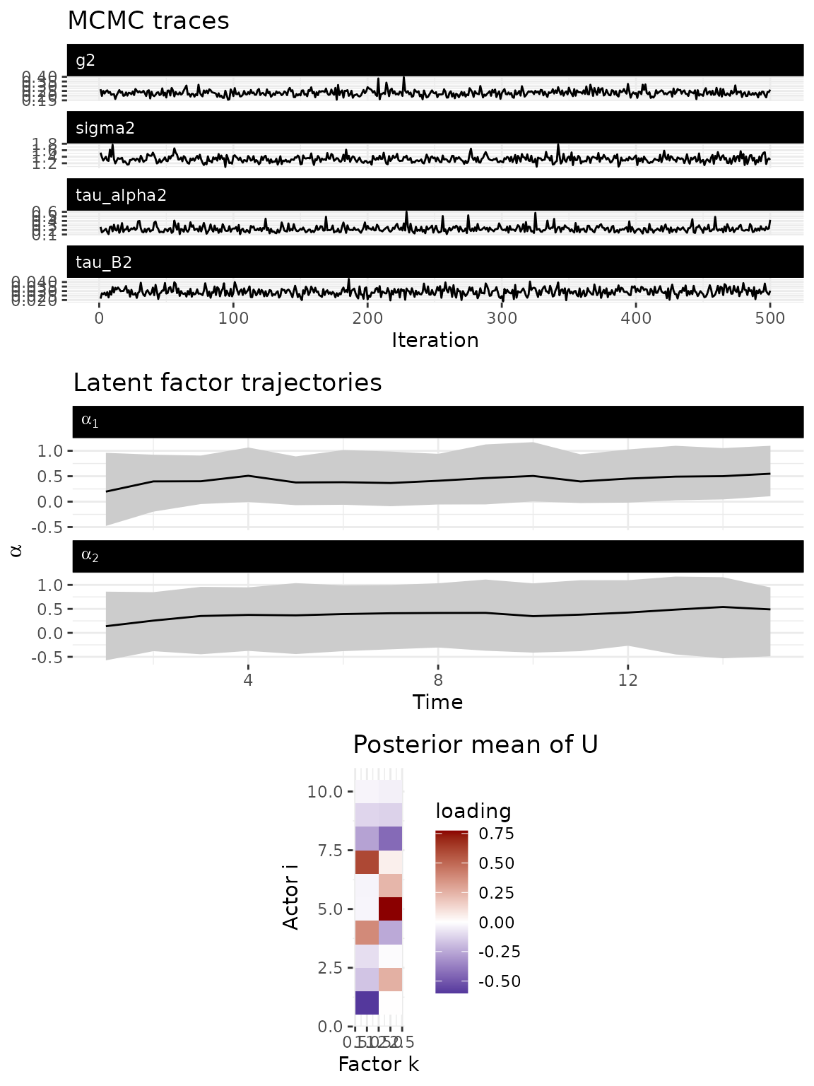

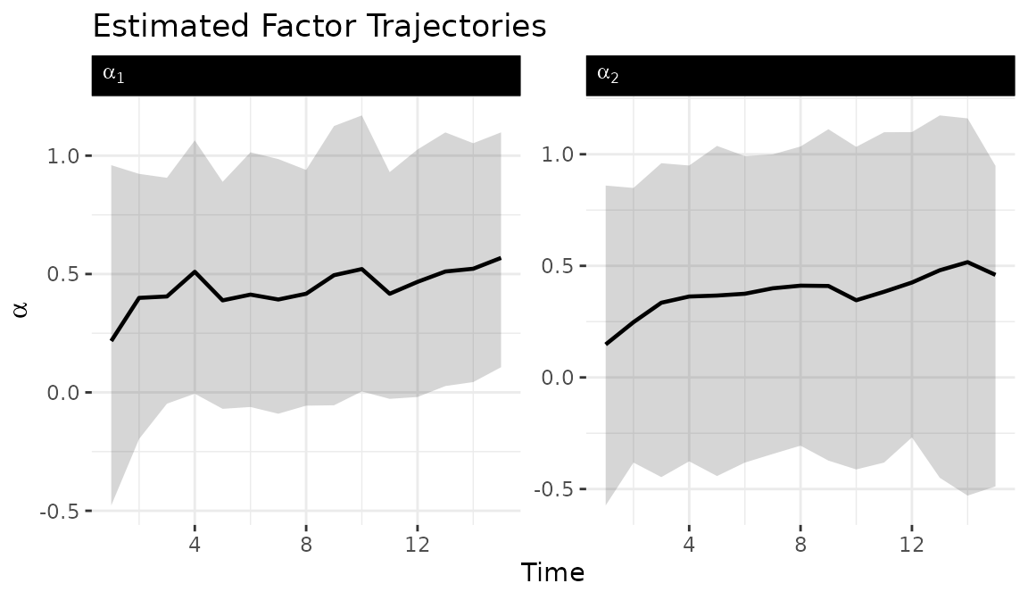
7 Factor trajectories

The tidy_dbn_lowrank() function extracts factor trajectories in tidy format for custom visualization. Ribbons show 95% posterior credible intervals.

alpha_df = tidy_dbn_lowrank(fit)

ggplot(alpha_df, aes(x = time, y = mean)) +
  geom_ribbon(aes(ymin = lo, ymax = hi), alpha = 0.2) +
  geom_line(linewidth = 0.8) +
  facet_wrap(
    ~ factor, scales = "free_y",
    labeller = label_bquote(alpha[.(factor)])
  ) +
  labs(
    title = "Estimated Factor Trajectories",
    x = "Time", y = expression(alpha)
  ) +
  theme_bw() +
  theme(
    panel.border = element_blank(),
    strip.background = element_rect(fill = "black", color = "black"),
    strip.text.x = element_text(color = "white", hjust = 0)
  )

8 Model summary

summary(fit)
#> Low-rank Dynamic Bilinear Network model
#>   nodes     : 10 
#>   relations : 1 
#>   time pts  : 15 
#>   rank      : 2 
#> 
#>            mean  2.5%  97.5%
#> sigma2     1.328 1.163 1.531
#> tau_alpha2 0.224 0.134 0.396
#> tau_B2     0.029 0.022 0.038
#> g2         0.229 0.177 0.299

9 Forecasting

Forecasts propagate both the factor dynamics $\alpha_t$ and the receiver dynamics $B_t$ forward, generating forecast distributions that reflect uncertainty in all model parameters.

pred = predict(fit, H = 3, draws = 100, summary = "mean")
dim(pred)
#> [1] 10 10  1  3

10 Choosing the rank

Start with $r = \lceil \log_2(n) \rceil$ and increase if posterior predictive checks show poor fit. Compare models with different ranks using compare_dbn(). Factors whose $\alpha_t$ trajectories remain near zero throughout the time series contribute little and suggest a lower rank suffices.

11 Next steps

For the full dynamic model without low-rank constraints, see vignette("dynamic_dbn"). For impulse response analysis, see vignette("impulse_response"). For the mathematical framework underlying all model variants, see vignette("methodology").

Tosin Salau & Shahryar Minhas

2026-03-28