Dynamic Effects in Longitudinal AME Models

Cassy Dorff, Tosin Salau, Shahryar Minhas

2026-07-25

Introduction

Networks change. Allies drift apart, tastes evolve. The standard AME model pools across time, assuming each actor has a fixed latent position and fixed additive effects in every period. The lame package provides three mechanisms for relaxing that assumption: dynamic_uv for time-varying latent positions, dynamic_ab for time-varying additive effects, and dynamic_beta for time-varying regression coefficients. This vignette explains what each option does, when to use it, and how to interpret the results.

What Are Dynamic Effects?

The Static Baseline

In the standard AME model for longitudinal data, the tie between actors $i$ and $j$ at time $t$ is:

$$y_{ij,t} = \beta'x_{ij,t} + a_i + b_j + u_i'v_j + \epsilon_{ij,t}$$

The covariates ($x_{ij,t}$) can vary over time, but the sender effect $a_i$, the receiver effect $b_j$, and the latent positions $u_i$ and $v_j$ are constant: the model assumes a country’s position in the latent “sanctioning space” is the same in 1993 as in 2000.

Dynamic Latent Positions (dynamic_uv = TRUE)

When you set dynamic_uv = TRUE, each actor’s latent position evolves over time according to an AR(1) process:

$$U_{i,k,t} = \rho_{uv} \, U_{i,k,t-1} + \epsilon_{i,k,t}, \quad \epsilon_{i,k,t} \sim N(0, \sigma_{uv}^2)$$$$V_{j,k,t} = \rho_{uv} \, V_{j,k,t-1} + \eta_{j,k,t}, \quad \eta_{j,k,t} \sim N(0, \sigma_{uv}^2)$$

Note the innovation parameterisation: $\sigma_{uv}^2$ is the variance of the period-to-period innovation, not the marginal/stationary variance of $U_{i,k,t}$ (which is $\sigma_{uv}^2 / (1 - \rho_{uv}^2)$), and fit$sigma_uv holds posterior draws of the innovation standard deviation. The autoregressive parameter $\rho_{uv}$, estimated from the data, controls persistence: near 1 means positions change slowly, near 0 means they are essentially re-drawn each period. Use this when the underlying community structure is evolving – alliances shift, trading blocs realign.

Dynamic Additive Effects (dynamic_ab = TRUE)

When you set dynamic_ab = TRUE, the sender and receiver effects evolve the same way:

$$a_{i,t} = \rho_{ab} \, a_{i,t-1} + \epsilon_{i,t}, \quad \epsilon_{i,t} \sim N(0, \sigma_{ab}^2)$$$$b_{j,t} = \rho_{ab} \, b_{j,t-1} + \eta_{j,t}, \quad \eta_{j,t} \sim N(0, \sigma_{ab}^2)$$

The same innovation parameterisation applies: fit$sigma_ab holds draws of the innovation standard deviation, and the implied stationary variance $\sigma_{ab}^2 / (1 - \rho_{ab}^2)$ doubles as the prior on the initial state $a_{i,1}$. Substantively, dynamic_ab captures changes in how much an actor participates, not in who they connect with (that is dynamic_uv’s territory). The two can be used alone or together; dynamic_ab is often the place to start, since changes in overall activity are common and relatively easy to estimate.

Dynamic Regression Coefficients (dynamic_beta)

The third option lets the regression coefficients themselves evolve. With dynamic_beta = TRUE (or a subset like dynamic_beta = "dyad"), each selected coefficient follows an AR(1):

$$\beta_{k,t} = \rho_{\beta,b(k)} \, \beta_{k,t-1} + \epsilon_{k,t}, \quad \epsilon_{k,t} \sim N(0, \sigma_{\beta,b(k)}^2 \Lambda_{kk})$$

where $b(k)$ is the block of coefficient $k$ (intercept / dyad / row / col), so coefficients in a block share $\rho$ and $\sigma$, while the design-based scale $\Lambda_{kk}$ (a $g$-prior analogue) keeps each innovation variance commensurate with the data. The whole time path of $\beta$ is drawn jointly via forward-filter / backward-sample (FFBS; Carter & Kohn 1994). One storage difference from dynamic_uv / dynamic_ab: fit$sigma_beta and fit$rho_beta hold last-iteration scalars, while the full posterior draws live in fit$SIGMA_BETA and fit$RHO_BETA – summarise those (e.g. colMeans(fit$SIGMA_BETA)).

dynamic_beta accepts FALSE (default), TRUE (all coefficients), block shortcuts ("intercept", "dyad", "row", "col") or coefficient names, integer column indices, or a length-p logical mask; see ?lame. When the intercept (or a nodal coefficient) is dynamic, an automatic sum-to-zero constraint on a (and b) keeps everything jointly identified. dynamic_beta works for every family, unipartite and bipartite, directed and symmetric, and combines with dynamic_ab / dynamic_uv.

A worked dynamic_beta example

Simulate a small longitudinal network where a single dyadic covariate’s effect grows linearly over time, and fit with dynamic_beta = "dyad".

library(lame)
set.seed(2026)

n_db <- 15
T_db <- 5
beta_t_true <- seq(-0.5, 1.0, length.out = T_db)   # truth: rising effect

X_db <- replicate(T_db, matrix(rnorm(n_db * n_db), n_db, n_db), simplify = FALSE)
Y_db <- vector("list", T_db)
for (t in seq_len(T_db)) {
    Yt <- beta_t_true[t] * X_db[[t]] + matrix(rnorm(n_db * n_db, 0, 0.4), n_db, n_db)
    diag(Yt) <- NA
    rownames(Yt) <- colnames(Yt) <- paste0("a", seq_len(n_db))
    Y_db[[t]] <- Yt
}
names(Y_db) <- paste0("t", seq_len(T_db))
X_db_arr <- lapply(X_db, function(x) array(x, c(n_db, n_db, 1)))

fit_db <- lame(Y_db, Xdyad = X_db_arr,
               family = "normal", R = 0,
               nscan = 200, burn = 50, odens = 5,
               dynamic_beta = "dyad", verbose = FALSE)

# fit$BETA is a 3-D array [n_stored x p x T]
dim(fit_db$BETA)
#> [1] 40  2  5

# coef() returns a p x T matrix of posterior means
coef(fit_db)
#>                    t1          t2          t3          t4          t5
#> intercept -0.00810071 -0.00810071 -0.00810071 -0.00810071 -0.00810071
#> X1_dyad   -0.48797080 -0.12866840  0.23813546  0.63432234  0.99248965

# confint() returns one row per coef[t] with 95% credible interval
head(confint(fit_db), 8)
#>                      2.5%       97.5%
#> intercept[t1] -0.03237708  0.01673393
#> X1_dyad[t1]   -0.52464259 -0.44517349
#> intercept[t2] -0.03237708  0.01673393
#> X1_dyad[t2]   -0.16936531 -0.08189014
#> intercept[t3] -0.03237708  0.01673393
#> X1_dyad[t3]    0.20885246  0.27956162
#> intercept[t4] -0.03237708  0.01673393
#> X1_dyad[t4]    0.58070472  0.68104416

Migration warning for amen / static-lame users. With dynamic_beta active, fit$BETA becomes a 3-D [n_stored, p, T] array rather than the 2-D [n_stored, p] matrix. The amen-era idiom apply(fit$BETA, 2, mean) still returns a length-p vector – but it now silently averages across both iterations and time, hiding the time variation you fit the model to recover. Use coef(fit) instead: it returns a [p, T] matrix for dynamic fits and a length-p vector for static ones.

The per-period posterior mean for X1_dyad should track the linear ramp beta_t_true = c(-0.5, -0.125, 0.25, 0.625, 1.0), with the AR(1) prior providing mild shrinkage relative to fitting a separate ame() per period.

Choosing a prior family: dynamic_beta_kind

lame() exposes dynamic_beta_kind for selecting the prior family on the time-varying coefficients:

Mean-reverting coefficient? Use the default dynamic_beta_kind = "ar1". Permanent / unit-root drift (no mean reversion)? Use "rw1". Smooth with curvature (second-order smoothness)? Use "rw2". Smooth with a known length-scale of variation? Use "matern32" (set the scale via prior = list(matern32_length_scale = ...); defaults to max(2, T/4)). If the stationarity warning fires after fitting AR(1) – the posterior on $\rho_\beta$ concentrated at or above 0.97 – refit with "rw1" (or "rw2" if acceleration matters).

"random_walk" is an alias for "rw1"; the "rw2" and "matern32" samplers use a slower R-level joint Gaussian update rather than the C++ FFBS. Refitting fit_db under each kind and comparing the recovered X1_dyad path against the truth:

kinds <- c("rw1", "rw2", "matern32")
paths <- sapply(kinds, function(k) {
    fit_k <- lame(Y_db, Xdyad = X_db_arr, family = "normal", R = 0,
                  nscan = 200, burn = 50, odens = 5,
                  dynamic_beta = "dyad", dynamic_beta_kind = k,
                  prior = if (k == "matern32")
                    list(matern32_length_scale = 2) else NULL,
                  verbose = FALSE)
    coef(fit_k)["X1_dyad", ]
})
round(rbind(ar1 = coef(fit_db)["X1_dyad", ], t(paths),
            truth = beta_t_true), 3)
#>              t1     t2    t3    t4    t5
#> ar1      -0.488 -0.129 0.238 0.634 0.992
#> rw1      -0.488 -0.126 0.230 0.638 0.988
#> rw2      -0.482 -0.123 0.224 0.624 0.999
#> matern32 -0.476 -0.124 0.223 0.627 0.989
#> truth    -0.500 -0.125 0.250 0.625 1.000

All four kinds recover essentially the same ramp – the point to take away, not a tie-breaker: on a smooth, gap-free trend the priors are nearly indistinguishable in-sample, and they diverge only when the data match their assumption. Choose with the decision tree above and the post-fit stationarity warning, not by eyeballing this table.

When time_index is supplied with unequal gaps, the AR(1) / RW1 conditional variance is scaled by the gap (suppressing $\Lambda_{kk}$ for readability): $$q_t = \sigma_\beta^2 \cdot \frac{1 - \rho_\beta^{2\Delta_t}}{1 - \rho_\beta^2}$$ so quarterly-then-annual data gets the correct prior; "rw2" and "matern32" support unequal gaps through their joint precision-matrix construction.

# observations at t = 1, 2, 4, 8 (a doubling gap structure)
fit_gaps <- lame(Y_db, Xdyad = X_db_arr, family = "normal", R = 0,
                 nscan = 200, burn = 50, odens = 5,
                 dynamic_beta = "dyad",
                 time_index = c(1, 2, 4, 8, 16)[seq_len(T_db)],
                 verbose = FALSE)
fit_gaps$time_index
#> [1]  1  2  4  8 16
round(coef(fit_gaps), 3)
#>               t1     t2     t3     t4     t5
#> intercept -0.011 -0.011 -0.011 -0.011 -0.011
#> X1_dyad   -0.485 -0.124  0.225  0.625  0.997

Hierarchical pooling: dynamic_beta_pool

When two or more coefficient blocks are dynamic, each block has its own AR(1) hyperparameters by default, and short panels ($T \le 5$) can leave them badly under-identified. dynamic_beta_pool shrinks block-level hyperparameters toward a shared mean: "rho" for common persistence, "sigma" for a common innovation scale, "both" for full pooling – e.g. lame(..., dynamic_beta = c("intercept", "dyad"), dynamic_beta_pool = "both"). With a single dynamic block the hierarchical layer is skipped entirely and the fit is identical to the default "none". See ?lame for the diagnostic comparison of pooled vs independent hyperparameter posteriors.

Per-actor time-varying slopes: dynamic_beta_per_actor

For questions about whether one actor responds to a covariate differently than another – and whether that gap evolves – set dynamic_beta_per_actor = "row" (or "col") and pick the covariate via per_actor_covariate_idx, e.g. lame(..., dynamic_beta_per_actor = "row", per_actor_covariate_idx = 1L). Deviations are sum-to-zero centred at every period, so the population coefficient stays in coef(fit) while the per-actor deviations land in fit$THETA_ACTOR (and their posterior means in fit$theta_actor_mean, labelled by actor and period). See ?per_actor_slopes.

Diagnosing your dynamic fit

summary(fit) prints the Dynamic coefficients per period block and the per-block posterior-mean rho_beta, and warns when a block’s posterior on $\rho_\beta$ is concentrated at or above 0.97 – the signal to refit with dynamic_beta_kind = "rw1".

detect_change_point(fit, threshold_bf = 5) is a heuristic regime-switch diagnostic: it scales each coefficient’s largest one-period jump by $\sigma_\beta$ and compares it to a prior-null reference, reporting a bounded tail-ratio score in the bf column (not a formal Bayes factor). On the smooth linear ramp above there is no break, so we expect a score of 0:

detect_change_point(fit_db, threshold_bf = 5)
#>      coef bf m_post_mean m_prior_q95 t_hat  warn
#> 1 X1_dyad  0   0.7297556    2.767291     4 FALSE

Read bf below 3 as weak, 3 to 10 as worth inspecting, and above 10 as a jump the AR(1) prior struggles to generate; t_hat is a prompt for visual inspection, not a formal break-time estimate. The diagnostic is deliberately conservative (only stark breaks trip it reliably at short $T$); see ?detect_change_point. For prior elicitation before fitting, dynamic_beta_prior_summary(T = 10, kind = "ar1") simulates prior paths so you can check the implied roughness and range for your T.

Finally, the Gibbs analog of HMC divergences: every fit exposes per-block Metropolis failure counts as fit$mh_counters, and a warning fires automatically when any block exceeds a 10% failure rate. Treat anything above 5% as suspicious.

Temporal-trend posterior-predictive check: gof_temporal()

Where detect_change_point() targets coefficients, gof_temporal(fit, stat = "density", n_rep = 200) targets the network statistic itself: it fits a linear time trend to a chosen statistic (density / mean / reciprocity / transitivity), computes the same slope on simulate(fit) replicates, and returns a two-sided posterior-predictive p-value; small p_pp (below 0.05) means the observed trend is incompatible with the fitted model. Reach for it when the substantive statistic drifts across the panel; the informative worked example lives in the overview vignette; see ?gof_temporal.

Inspecting the priors actually in effect: prior_summary()

prior_summary(fit) prints the hyperparameters actually used, defaults filled in – for a dynamic fit that includes the per-block AR(1) priors alongside the variance components and the g-prior on beta. Run it once per fit to catch typos in a prior = list(...) override; see ?prior_summary and the cross-sectional vignette for the general tour.

Multi-chain $\hat R$ via lame_parallel() and rhat_dynamic_beta()

A single chain only ever buys you within-chain split-$\hat R$. For a between-chain diagnostic on the per-period coefficient path, fit several chains with lame_parallel(..., n_chains = 4, combine_method = "list") and call rhat_dynamic_beta() on the resulting list. Require both rhat_mvt < 1.01 (the multivariate statistic catches chains that agree per period but disagree on the trajectory) and rhat_max_univariate < 1.01 before quoting a path; short vignette-length chains typically fail this bar, so use production lengths. combine_ame_chains() pools chains and routes through posterior::summarise_draws() for per-(coefficient, period) ESS. ame_parallel() is the cross-sectional twin; see ?rhat_dynamic_beta, ?lame_parallel, and the cross-sectional vignette.

Forecasting

When at least one dynamic component is active, predict(fit, h = K) propagates the state-space model forward $K$ periods, sampling $(\rho_\beta, \sigma_\beta)$ from the posterior so the forecast carries hyperparameter uncertainty. The forecasting vignette is the full worked reference (forecast scales, per-draw arrays, credible intervals, counterfactual covariates, exposure offsets, near-unit-root warning). One kind-specific note lives here: under "rw2" / "matern32" the forward recursion pins $\rho_\beta$ at 1, so forecast variance grows linearly in $h$ as under RW1 – the smoothing structure shapes the in-sample path only.

Visualising the coefficient path: autoplot.lame

For a fit with dynamic_beta active, autoplot(fit) returns a ggplot ribbon plot per coefficient (posterior median line, 95% interval, faceted by coefficient). Under dynamic_beta = "dyad" the intercept remains static, so pass coefs = to restrict the plot to the genuinely time-varying coefficients:

library(ggplot2)
autoplot(fit_db, coefs = "X1_dyad", probs = c(0.025, 0.5, 0.975)) +
    labs(title = "Posterior coefficient path",
         subtitle = "Median line, 95% credible interval ribbon",
         x = "Time period", y = "Coefficient value")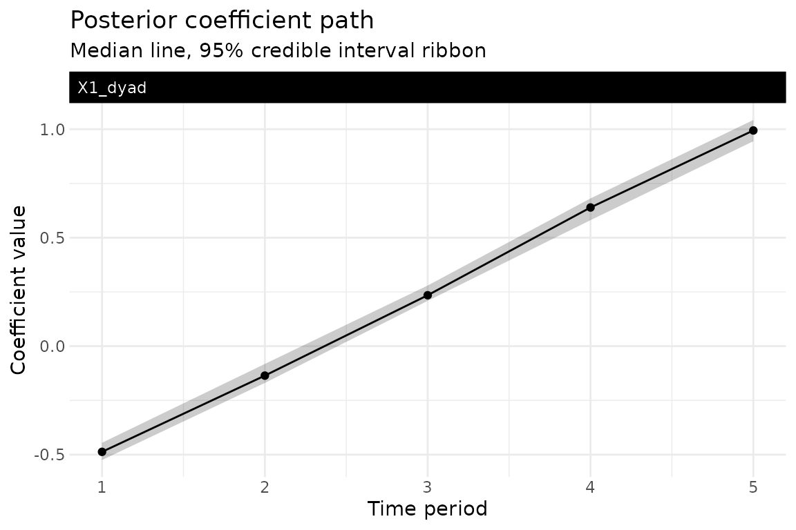

LOO / WAIC via save_log_lik = TRUE

Pass save_log_lik = TRUE and lame attaches a [n_stored, n_obs] pointwise log-likelihood matrix to fit$log_lik, which registered S3 methods hand directly to loo::loo(fit) and loo::waic(fit):

fit_ll <- lame(Y_db, Xdyad = X_db_arr, family = "normal", R = 0,
               nscan = 2000, burn = 500, odens = 25,
               dynamic_beta = "dyad",
               save_log_lik = TRUE,
               verbose = FALSE)

dim(fit_ll$log_lik)        # [n_stored, n_observations]
loo_db <- loo::loo(fit_ll)
print(loo_db)

The code is left unevaluated because a useful PSIS-LOO calculation needs more draws than a vignette should generate. Run it with a converged fit before using elpd_loo. If the matrix would not fit in RAM, save_log_lik = "chunked" streams it to disk (see the forecasting vignette).

On the log-likelihood scale: for normal, binary, cbin, poisson, and ordinal the stored pointwise log-likelihood is the exact family-specific Y density on the response scale, so elpd_loo is directly comparable to a Stan / brms loo() on the same family and data (modulo satisfactory $\hat R$ / ESS). For the rank likelihood frn, the exact marginal needs GHK Monte Carlo (log_lik_method = "observed_ghk", longitudinal path only); the default falls back to the augmented-Z normal density with a one-time warning. Inspect fit$log_lik_method for the branch used.

Prior Specifications

The AR(1) coefficients and innovation variances have sensible default priors:

• $\rho_{uv} \sim \text{TruncNormal}(0.9, 0.1, 0, 1)$, centered on high persistence
• $\rho_{ab} \sim \text{TruncNormal}(0.8, 0.15, 0, 1)$, slightly less persistent
• $\rho_{\beta} \sim \text{TruncNormal}(0.8, 0.15, 0, 0.999)$
• $\sigma_{uv}^2, \sigma_{ab}^2, \sigma_{\beta}^2 \sim \text{InverseGamma}(2, 1)$

All can be customized via the prior argument (e.g. prior = list(rho_beta_mean = ..., sigma_beta_scale = ...)) if you have strong beliefs about the rate of change.

Genuine Dynamics: What They Look Like

We start with an example where dynamics are truly present: 25 actors over 5 periods whose latent positions evolve via an AR(1) with $\rho = 0.85$ and innovation SD $\sigma_{uv} = 0.3$. Initial positions are drawn at SD 1.5 – above the implied stationary SD of about 0.57 – seeding strong latent structure that drifts toward stationarity, with a negative intercept giving realistic density (roughly 30%).

library(lame)
set.seed(6886)

n_dyn <- 25
n_per <- 5
R_dyn <- 2

# evolving latent positions with AR(1) dynamics
U <- matrix(rnorm(n_dyn * R_dyn, 0, 1.5), n_dyn, R_dyn)
V <- matrix(rnorm(n_dyn * R_dyn, 0, 1.5), n_dyn, R_dyn)

Y_dyn <- list()
for(t in 1:n_per) {
    if(t > 1) {
        U <- 0.85 * U + matrix(rnorm(n_dyn * R_dyn, 0, 0.3), n_dyn, R_dyn)
        V <- 0.85 * V + matrix(rnorm(n_dyn * R_dyn, 0, 0.3), n_dyn, R_dyn)
    }
    eta <- -1 + U %*% t(V)
    Y_t <- matrix(rbinom(n_dyn * n_dyn, 1, pnorm(eta)), n_dyn, n_dyn)
    diag(Y_t) <- NA
    rownames(Y_t) <- colnames(Y_t) <- paste0("A", 1:n_dyn)
    Y_dyn[[t]] <- Y_t
}

# iterations are small so the vignette builds quickly
# use burn >= 1000 and nscan >= 5000 for real analyses.
fit_dyn_real <- lame(Y_dyn, R = 2,
    dynamic_uv = TRUE, dynamic_ab = TRUE,
    family = "binary",
    burn = 100, nscan = 1000, odens = 10,
    verbose = FALSE, plot = FALSE)

summary(fit_dyn_real)
#> 
#> === Longitudinal AME Model Summary ===
#> 
#> Call:
#> [1] "Y ~ a[i] + b[j] + rho*e[ji] + U[i,1:2] %*% V[j,1:2], family = 'binary'"
#> 
#> Time periods: 5 
#> Family: binary 
#> Mode: unipartite 
#> Dynamic latent positions: enabled (rho_uv = 0.963 )
#> Dynamic additive effects: enabled (rho_ab = 0.606 )
#> 
#> Regression coefficients:
#> ------------------------
#>           Estimate StdError z_value p_value CI_lower CI_upper    
#> intercept   -1.066     0.06 -17.662       0   -1.175    -0.94 ***
#> ---
#> Signif. codes: 0 '***' 0.001 '**' 0.01 '*' 0.05 '.' 0.1 ' ' 1
#> Note: stars are a visual hint from posterior mean / SD only; for inference use the credible intervals.
#> 
#> Variance components:
#> -------------------
#>     Estimate StdError
#> va     0.092    0.042
#> cab   -0.007    0.025
#> vb     0.109    0.044
#> rho   -0.055    0.068
#> ve     1.000    0.000
#>   (va = sender, cab = sender-receiver covariance, vb = receiver,
#>    rho = dyadic correlation, ve = residual variance)

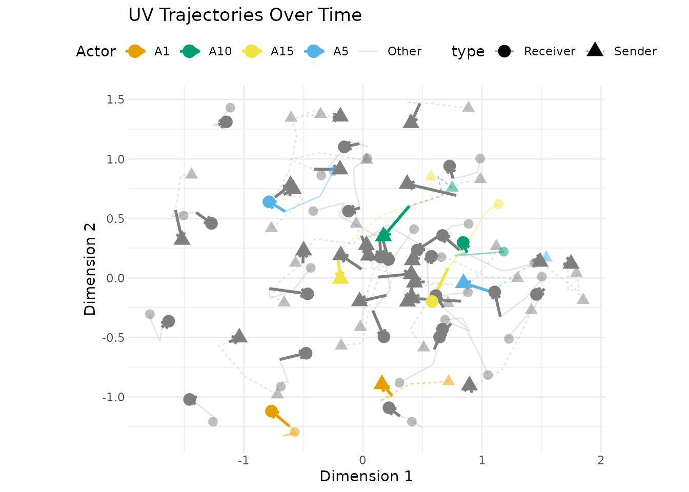
The trajectory plot shows how actors move through the latent space. With more than eight actors the legend becomes an unreadable rainbow, so pass highlight = a few actor names to grey out the rest (colour-blind-safe Okabe–Ito palette for the highlighted set). With genuine temporal structure, the highlighted paths trace short, coherent arcs rather than random jumps:

uv_plot(fit_dyn_real, plot_type = "trajectory",
        highlight = c("A1", "A5", "A10", "A15"))

Always check convergence: dynamic models have more parameters than static ones, so adequate mixing requires longer chains. Under the binary (probit) family the error variance ve is fixed at 1 for identification, so exclude it by its display label:

trace_plot(fit_dyn_real, exclude = "Error Variance")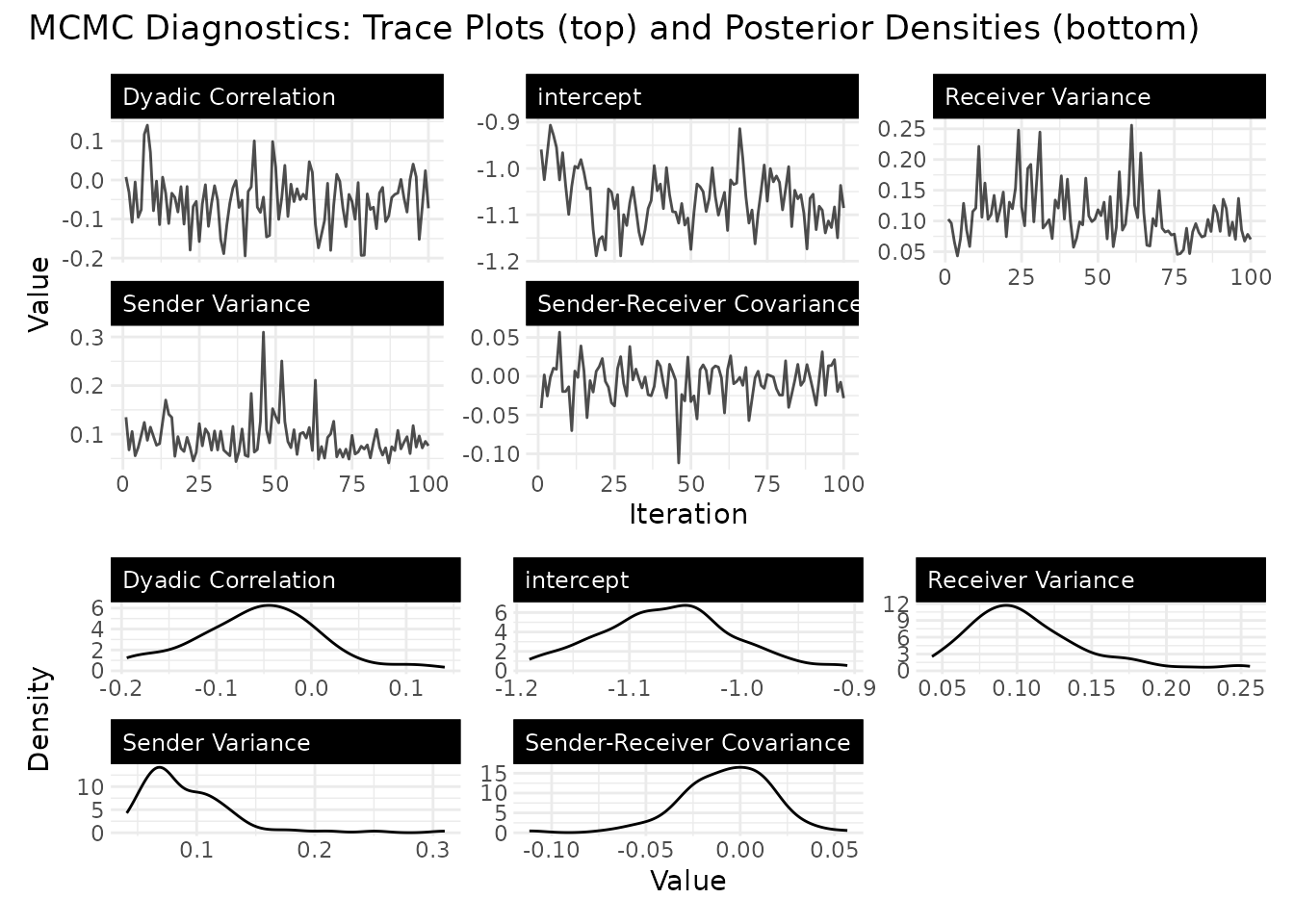

What Happens Without Temporal Structure?

To see how the dynamic model behaves when there is no signal, we fit the same model to independent networks – a null baseline showing what the prior alone produces when the data are uninformative.

set.seed(6886)
n <- 30
n_periods <- 5

# independent binary networks with no temporal structure
Y_list <- list()
for(t in 1:n_periods) {
    Y_t <- matrix(rbinom(n*n, 1, 0.2), n, n)
    diag(Y_t) <- NA
    rownames(Y_t) <- colnames(Y_t) <- paste0("Actor", 1:n)
    Y_list[[t]] <- Y_t
}

# fit with a custom prior on rho_uv to illustrate prior sensitivity
prior_custom <- list(
    rho_uv_mean = 0.95,    # expect very slow change in latent positions
    rho_uv_sd = 0.05       # tight prior
)

fit_null <- lame(
    Y = Y_list,
    R = 2,
    dynamic_uv = TRUE,
    dynamic_ab = TRUE,
    family = "binary",
    prior = prior_custom,
    burn = 100,
    nscan = 1000,
    odens = 10,
    # save per-draw latent trajectories for latent_positions() /
    # procrustes_align(per_draw = TRUE) below
    posterior_opts = list(save_UV = TRUE),
    verbose = FALSE,
    plot = FALSE
)

summary(fit_null)
#> 
#> === Longitudinal AME Model Summary ===
#> 
#> Call:
#> [1] "Y ~ a[i] + b[j] + rho*e[ji] + U[i,1:2] %*% V[j,1:2], family = 'binary'"
#> 
#> Time periods: 5 
#> Family: binary 
#> Mode: unipartite 
#> Dynamic latent positions: enabled (rho_uv = 0.799 )
#> Dynamic additive effects: enabled (rho_ab = 0.373 )
#> 
#> Regression coefficients:
#> ------------------------
#>           Estimate StdError z_value p_value CI_lower CI_upper    
#> intercept   -0.911    0.027  -33.44       0   -0.956   -0.857 ***
#> ---
#> Signif. codes: 0 '***' 0.001 '**' 0.01 '*' 0.05 '.' 0.1 ' ' 1
#> Note: stars are a visual hint from posterior mean / SD only; for inference use the credible intervals.
#> 
#> Variance components:
#> -------------------
#>     Estimate StdError
#> va     0.046    0.014
#> cab   -0.002    0.010
#> vb     0.045    0.013
#> rho    0.070    0.043
#> ve     1.000    0.000
#>   (va = sender, cab = sender-receiver covariance, vb = receiver,
#>    rho = dyadic correlation, ve = residual variance)

We can compare the estimated persistence parameters across the two settings:

cat("Independent data rho_uv:", round(mean(fit_null$rho_uv), 3), "\n")
#> Independent data rho_uv: 0.799
cat("Correlated data rho_uv:", round(mean(fit_dyn_real$rho_uv), 3), "\n")
#> Correlated data rho_uv: 0.963

Even with a deliberately tight prior centred at 0.95, the two posteriors diverge: the correlated fit lands in the upper AR(1) range (expect small-sample upward bias at $T = 5$, so the posterior can sit above the true 0.85), while the null fit collapses well below the prior centre because the data carry no period-to-period correlation to anchor against. The AR(1) parameter does real work even on a modest panel, but the point estimate of rho_uv is no substitute for the trajectory plots (compare the coherent paths above with the erratic paths below).

Visualizing the Null Case

The trajectory plot for independent data looks different. Using the same highlight device as above, the highlighted paths jump from period to period without persistent direction, and the whole cloud clumps near the origin:

uv_plot(fit_null, plot_type = "trajectory",
        highlight = c("Actor1", "Actor5", "Actor10", "Actor15"))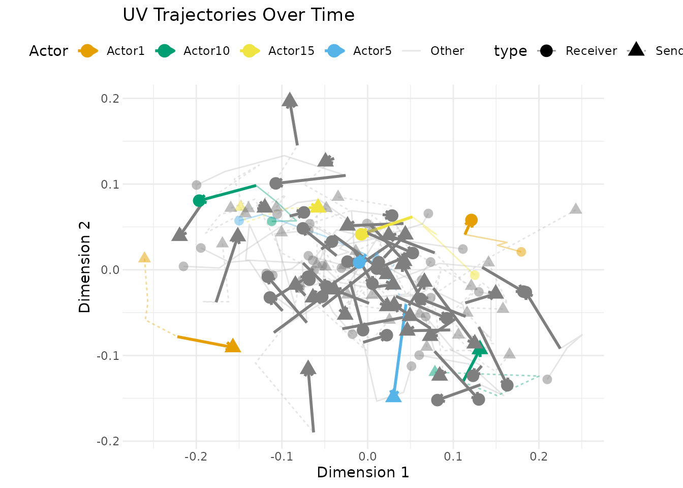

The additive effects behave the same way: trajectories reflecting noise rather than real shifts in actor activity.

ab_plot(fit_null, effect = "sender", plot_type = "trajectory")
#> ℹ Showing top 5 and bottom 5 actors by average effect
#> → Use `show_actors` to specify actors to display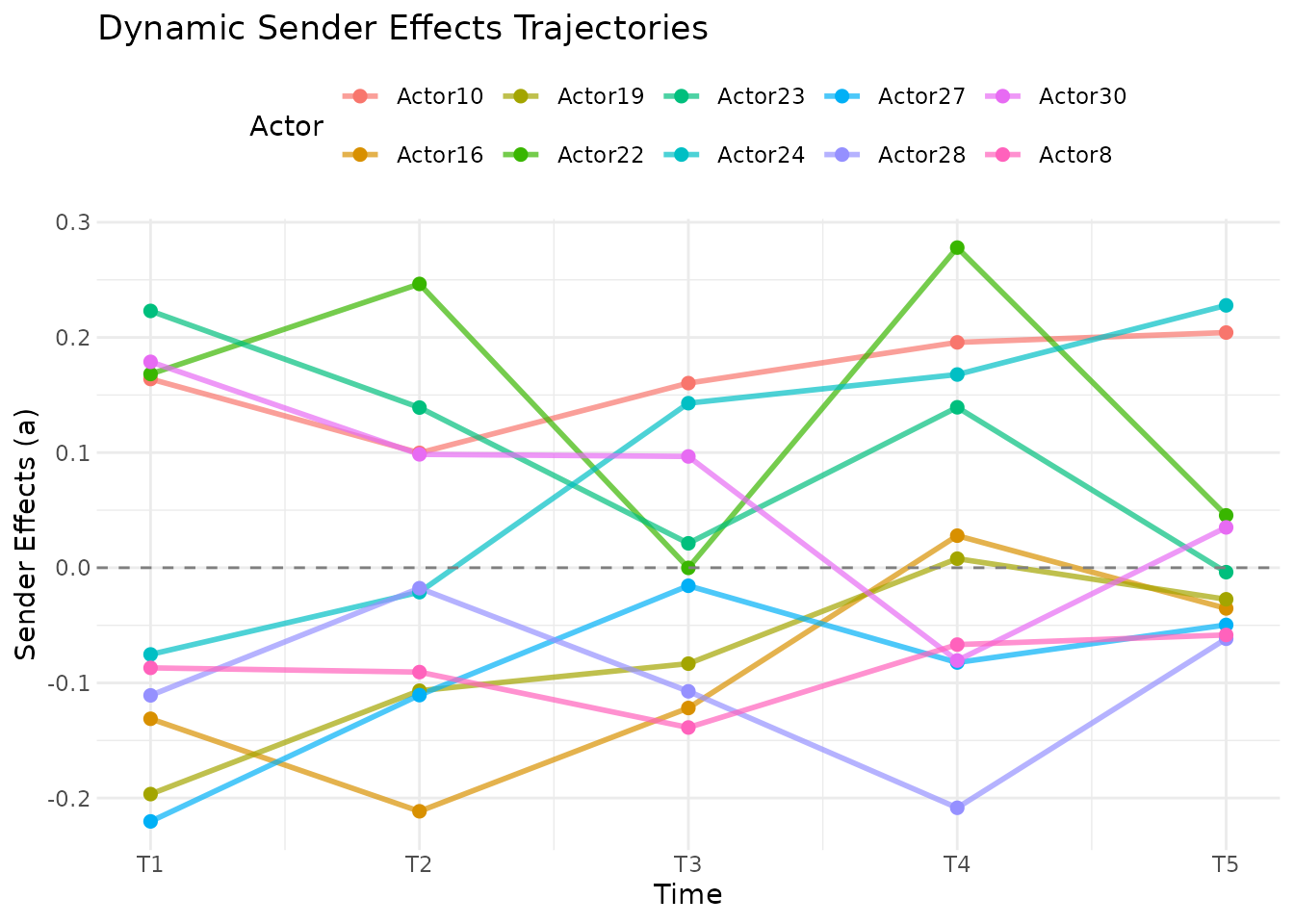

Comparing Model Specifications

A natural workflow is to fit several specifications and compare their goodness-of-fit. We use the independent data from above, where dynamic effects should add nothing.

# four small fits to compare specifications. nscan is intentionally
# small here so the vignette stays under CRAN's vignette compute
# budget; for a real comparison use nscan >= 2000 per fit and run them
# under `ame_parallel()` with 4 chains.
fit_static <- lame(Y_list, R = 2, family = "binary",
                                    burn = 30, nscan = 150, odens = 5,
                                    verbose = FALSE, plot = FALSE)

fit_uv <- lame(Y_list, R = 2, dynamic_uv = TRUE, family = "binary",
                            burn = 30, nscan = 150, odens = 5,
                            verbose = FALSE, plot = FALSE)

fit_ab <- lame(Y_list, R = 2, dynamic_ab = TRUE, family = "binary",
                            burn = 30, nscan = 150, odens = 5,
                            verbose = FALSE, plot = FALSE)

fit_full <- lame(Y_list, R = 2, dynamic_uv = TRUE, dynamic_ab = TRUE,
                                family = "binary",
                                burn = 30, nscan = 150, odens = 5,
                                verbose = FALSE, plot = FALSE)

For each specification we compute posterior predictive p-values (how often simulated statistics exceed observed): values near 0.5 indicate good fit; values pinned near 0 or 1 flag a statistic the model systematically under- or over-generates.

# compute p-values for each model and each GOF statistic
compute_pvals <- function(fit) {
    gof <- fit$GOF
    sapply(names(gof), function(stat) {
        mat <- gof[[stat]]
        obs <- mat[, 1]           # first column = observed
        sims <- mat[, -1]         # remaining = posterior predictive
        mean(colMeans(sims) >= mean(obs))
    })
}

gof_comparison <- rbind(
    Static     = compute_pvals(fit_static),
    Dynamic_UV = compute_pvals(fit_uv),
    Dynamic_AB = compute_pvals(fit_ab),
    Full       = compute_pvals(fit_full)
)
round(gof_comparison, 3)
#>            sd.rowmean sd.colmean dyad.dep cycle.dep trans.dep
#> Static          0.967      0.967    0.433     0.500     0.333
#> Dynamic_UV      0.933      0.933    0.533     0.467     0.400
#> Dynamic_AB      1.000      1.000    0.533     0.533     0.400
#> Full            1.000      1.000    0.367     0.667     0.367

sd.rowmean and sd.colmean sit near 1 for every specification – an artifact of fitting a heterogeneity model to homogeneous iid data, not evidence about dynamics – so compare specifications on the dyad.dep, cycle.dep, and trans.dep columns instead. There, no specification is clearly better, as expected for data generated without temporal structure; with short chains these p-values are noisy, so read the table as “the dynamic terms add nothing”, not as a ranking.

When to Use Dynamic Effects

Use dynamic_ab when actors’ overall activity levels change over time: countries cycle through isolationist and interventionist periods, users churn in and out of platforms.

Use dynamic_uv when the underlying community structure is shifting – a stronger claim: not just that actors are more or less active, but that who connects with whom is changing (political realignment, generational turnover).

Use dynamic_beta when a covariate’s effect on tie formation changes over time while actors and community structure are stable: the question is how strongly X translates into Y, not who is connecting (dynamic_uv) or who is active (dynamic_ab).

Use multiple together when several types of change happen at once – the most flexible but most data-hungry specification; with short panels or sparse networks the dynamic parameters may not be well-identified.

Stick with static when you have few time periods, when the network is genuinely stable, or when you primarily care about average covariate effects.

Dealing with Rotational Indeterminacy

One subtlety of dynamic latent space models: the latent space is only identified up to an orthogonal rotation at each time point and at each posterior draw. Even under smooth true dynamics, raw $U_t$ estimates can “jump” between periods, and posterior means can shrink toward zero across differently rotated draws. procrustes_align() applies the orthogonal-Procrustes rotation (Gower 1975) to align each period’s positions to the previous one:

# align latent positions across time
aligned <- procrustes_align(fit_null)
str(aligned$U)  # 3D array: actors x dimensions x time
#>  num [1:30, 1:2, 1:5] -0.26043 0.07856 0.06056 0.16564 0.00521 ...
#>  - attr(*, "dimnames")=List of 3
#>   ..$ : chr [1:30] "Actor1" "Actor10" "Actor11" "Actor12" ...
#>   ..$ : NULL
#>   ..$ : NULL

By default this aligns the posterior-mean trajectory fit$U across time only. Rotation indeterminacy is a per-draw property, though, so the stricter standard (Hoff 2005; Sewell & Chen 2015) is to align each posterior draw to a reference before summarising: procrustes_align(fit, per_draw = TRUE) does that on the per-draw cube a dynamic fit stores when you opt in via posterior_opts = list(save_UV = TRUE) – as we did for fit_null. Without the opt-in it falls back to mean-trajectory alignment with a note; see ?procrustes_align.

latent_positions(fit, align = TRUE) returns the aligned positions as a tidy data frame ready for ggplot2 (custom trajectory plots, overlaying external events). Because this fit saved its per-draw trajectories, the posterior_sd column is computed from the draws rather than returned as NA – though those SDs fold in some rotational wobble across draws:

lp <- latent_positions(fit_null, align = TRUE)
head(lp)
#>     actor dimension time        value posterior_sd type
#> 1  Actor1         1    1 -0.260429691    0.4699625    U
#> 2 Actor10         1    1  0.078562328    0.4704766    U
#> 3 Actor11         1    1  0.060560527    0.4019490    U
#> 4 Actor12         1    1  0.165641775    0.5317388    U
#> 5 Actor13         1    1  0.005207137    0.5112595    U
#> 6 Actor14         1    1 -0.034462647    0.4542168    U

References

1. Hoff, PD (2021). Additive and Multiplicative Effects Network Models. Statistical Science 36, 34–50.

2. Hoff, PD (2005). Bilinear mixed-effects models for dyadic data. Journal of the American Statistical Association 100(469), 286–295.

3. Sewell, D. K., & Chen, Y. (2015). Latent space models for dynamic networks. Journal of the American Statistical Association, 110(512), 1646-1657.

4. Carter, C. K., & Kohn, R. (1994). On Gibbs sampling for state space models. Biometrika 81(3), 541–553. The FFBS algorithm behind dynamic_beta_kind = "ar1" / "rw1".

5. Gower, J. C. (1975). Generalized Procrustes analysis. Psychometrika 40(1), 33–51. The orthogonal-Procrustes rotation underlying procrustes_align().