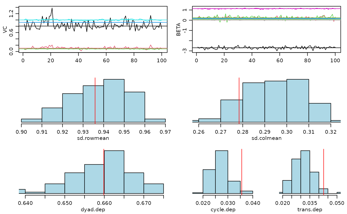
Simple diagnostic plot for AME model fit

Provides a quick visual summary of an AME model fit, focusing on key convergence diagnostics. For more detailed diagnostics, use the specific plotting functions: trace_plot(), gof_plot(), ab_plot(), and uv_plot().

Usage

# S3 method for class 'ame'
plot(x, ...)

Arguments

x: an object of class "ame" from fitting an AME model
...: additional arguments passed to trace_plot()

Value

A ggplot2 object from trace_plot() (invisibly)

Details

By default, this function simply calls trace_plot() to show MCMC trace plots and posterior distributions for key parameters. This provides a quick check of model convergence and mixing.

For more detailed visualizations, use the specialized functions:

trace_plot(): MCMC diagnostics and posterior distributions
gof_plot(): Goodness-of-fit assessment
ab_plot(): Additive sender/receiver effects
uv_plot(): Multiplicative latent factors

Author

Cassy Dorff, Shahryar Minhas, Tosin Salau

Examples

# \donttest{
# Fit an AME model
data(YX_nrm)
fit <- ame(YX_nrm$Y, Xdyad = YX_nrm$X, R = 2, gof = TRUE,
           nscan = 100, burn = 10, odens = 1, verbose = FALSE)

# Quick diagnostic plot (shows trace plots)
plot(fit)

# }