Plot diagnostics for a LAME model fit

Creates diagnostic plots for a LAME (Longitudinal Additive and Multiplicative Effects) model, including MCMC diagnostics, parameter evolution over time, and longitudinal goodness-of-fit checks. This is the default plot method for LAME objects.

Usage

# S3 method for class 'lame'
plot(
  x,
  which = c(1, 2, 3, 4),
  time.points = NULL,
  ask = FALSE,
  pages = c("single", "multiple"),
  ...
)

Arguments

x

an object of class "lame" from fitting a LAME model

which

numeric or character vector specifying which plots to produce: 1 or "trace" = MCMC trace plots, 2 or "density" = posterior density plots, 3 or "gof" = longitudinal goodness-of-fit plots, 4 or "effects" = additive and multiplicative effects, 5 or "network" = network snapshots at selected times. Default is c(1,2,3,4) to show main diagnostic plots.

time.points

numeric vector of time points for network snapshots (only used if "network" in which). Default is c(1, middle, last).

ask

logical; if TRUE, user is prompted before each plot page

pages

character string specifying how to arrange plots: "single" = one combined page (default), "multiple" = separate pages for each plot type

...

additional arguments (currently not used)

Value

NULL (invisibly). Plots are displayed as side effects.

Details

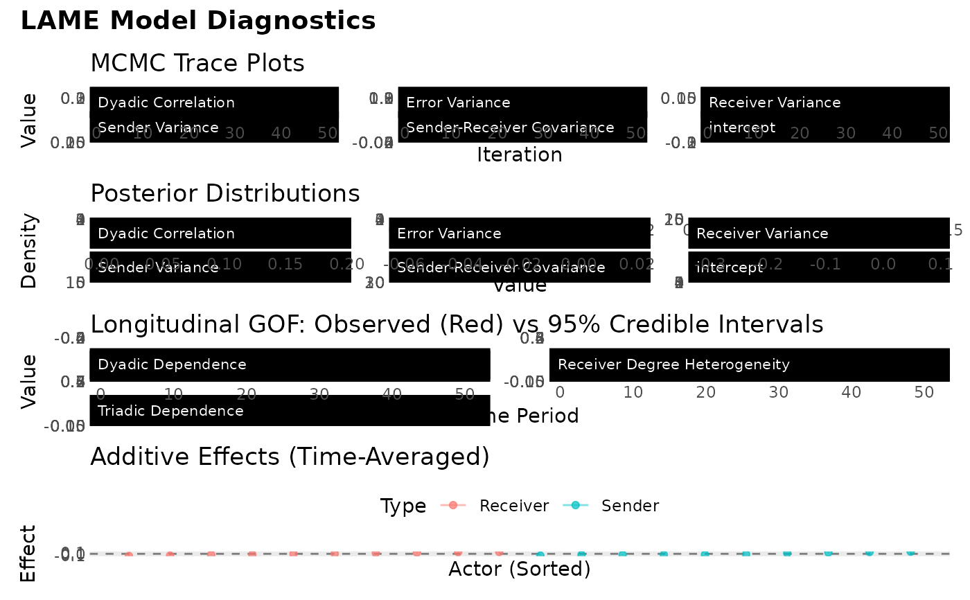
The function produces a multi-panel plot containing:

MCMC trace plots

Shows mixing and convergence of key parameters

Posterior distributions

Density plots of regression coefficients and variance components

Longitudinal GOF

Time series of observed network statistics with posterior predictive intervals

Effects over time

Evolution of additive effects across time periods (if applicable)

Network snapshots

Visualization of network at selected time points

The plot adapts to the longitudinal structure:

• Shows temporal trends in network statistics

• Highlights composition changes if actors enter/exit

• Displays credible intervals for time-varying statistics

See also

lame, trace_plot, gof_plot, ab_plot, uv_plot

Author

Cassy Dorff, Shahryar Minhas, Tosin Salau

Examples

# \donttest{
# Create simple longitudinal network data
set.seed(6886)
n <- 10
nms <- paste0("n", 1:n)
Y_list <- list(
  matrix(rnorm(n * n), n, n, dimnames = list(nms, nms)),
  matrix(rnorm(n * n), n, n, dimnames = list(nms, nms))
)
diag(Y_list[[1]]) <- diag(Y_list[[2]]) <- NA
fit <- lame(Y_list, family = "normal",
            nscan = 50, burn = 10, odens = 1, verbose = FALSE, plot = FALSE)

# default combined plot
plot(fit)
#> ℹ Generating LAME diagnostic plots: trace, density, gof, effects
#> ℹ Combining plots into single page layout

# }