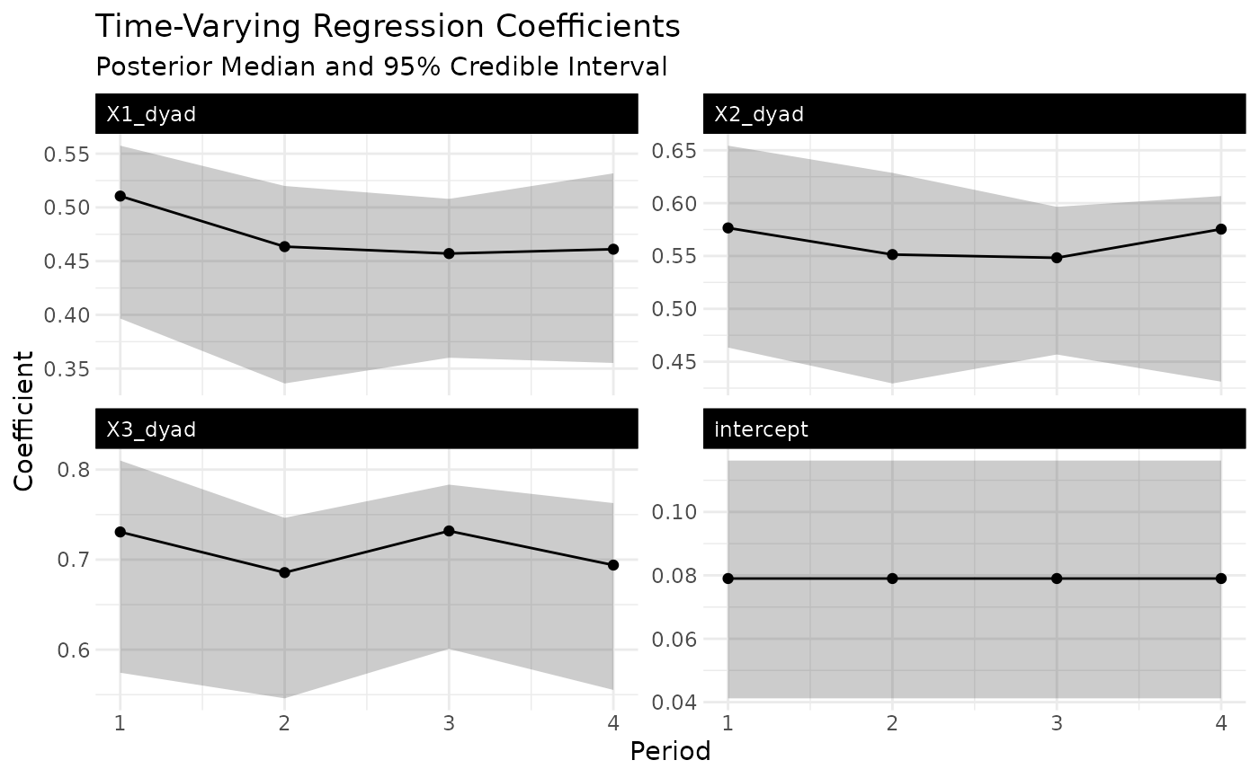
Ribbon plot of time-varying coefficients (or coefplot for static fits)

For a lame fit with dynamic_beta on, returns a faceted ggplot of the posterior mean coefficient path per period with a 95 percent credible-interval ribbon. For a static fit (no dynamic_beta), falls back to a tidy()-driven horizontal coefplot with posterior-mean point estimate and credible-interval bars so that autoplot(fit) returns a ggplot regardless of fit type.

Usage

# S3 method for class 'lame'
autoplot(
  object,
  which = c("beta", "ab", "uv"),
  probs = c(0.025, 0.5, 0.975),
  coefs = NULL,
  ...
)

# S3 method for class 'ame'
autoplot(
  object,
  which = c("beta", "ab", "uv"),
  probs = c(0.025, 0.5, 0.975),
  coefs = NULL,
  ...
)

Arguments

object

A fitted ame / lame object.

which

One of "beta" (default; coefficient plot – ribbon when dynamic, coefplot when static), "ab" (sender / receiver effects when dynamic_ab), "uv" (latent positions when dynamic_uv).

probs

Length-3 vector of quantiles to plot. Default c(0.025, 0.5, 0.975) for 95 percent intervals.

coefs

Optional character vector of coefficient names to subset.

...

Ignored.

Value

A ggplot2 object that can be further customised.

Examples

# \donttest{
data(YX_bin_list)
fit <- lame(YX_bin_list$Y, YX_bin_list$X, family = "binary", R = 0,
            dynamic_beta = "dyad",
            nscan = 60, burn = 15, odens = 5, verbose = FALSE)
#> Warning: `family` = "binary" but `Y` contains values other than 0/1.
#> ℹ `Y` will be thresholded to `1 * (Y > 0)`; if you meant counts, use "poisson",
#>   or "ordinal"/"normal" as appropriate.
if (requireNamespace("ggplot2", quietly = TRUE)) {
  autoplot(fit)
}

# }