Forecasting Longitudinal Networks with lame

Cassy Dorff, Tosin Salau, Shahryar Minhas

2026-07-25

What this vignette covers

lame() with at least one dynamic component (dynamic_beta, dynamic_ab, dynamic_uv) gives you a state-space model that is exactly the right object for forecasting future periods. This vignette walks through:

1. Fit a model with dynamic coefficients.
2. Forecast h periods ahead on the link scale and the response scale.
3. Compute counterfactual forecasts by feeding in alternative future covariates.
4. Visualise the forecast and the per-coefficient ribbon plot.
5. Diagnose whether the forecast variance has exploded (near- unit-root coefficients).

Step 1: Fit

Forecasting needs a fit where the dynamic coefficient is actually identified at each period, so we simulate a panel that delivers that: 30 actors over 6 periods, a single dyadic covariate trade, and a directed binary outcome cooperation. The effect of trade on cooperation is genuinely time-varying but mean-reverting – it follows an AR(1) around 0.5 with persistence 0.7, starting high (0.9) and settling toward its long-run level. The network is moderately dense (~37%), which is what makes per-period coefficients estimable; this is the regime in which forecasting is well-posed.

A note on data choice: dynamic_beta needs both a reasonable number of periods and enough ties per period to pin down a coefficient for that period. Very sparse panels (say a rare-event sanctions network at ~2% density over 3-4 years) do not carry that per-period information, the AR(1) persistence runs up against a unit root, and the forecast variance explodes (Step 5 shows exactly that failure mode). A simulated panel lets us show forecasting working before we show it failing.

library(lame)
set.seed(2026)

n_fc <- 30
T_fc <- 6
rho_true   <- 0.7
beta_bar   <- 0.5
beta_t_true <- numeric(T_fc)
beta_t_true[1] <- 0.9
for (t in 2:T_fc) {
    beta_t_true[t] <- beta_bar + rho_true * (beta_t_true[t - 1] - beta_bar) +
        rnorm(1, 0, 0.15)
}

Xdyad <- lapply(seq_len(T_fc), function(t) {
    x <- matrix(rnorm(n_fc * n_fc), n_fc, n_fc)
    array(x, dim = c(n_fc, n_fc, 1),
          dimnames = list(NULL, NULL, "trade"))
})
a_fc <- rnorm(n_fc, 0, 0.4)
b_fc <- rnorm(n_fc, 0, 0.4)
Y <- lapply(seq_len(T_fc), function(t) {
    eta <- -0.5 + beta_t_true[t] * Xdyad[[t]][, , 1] + outer(a_fc, b_fc, "+")
    Yt  <- matrix(rbinom(n_fc * n_fc, 1, pnorm(eta)), n_fc, n_fc)
    diag(Yt) <- NA
    rownames(Yt) <- colnames(Yt) <- sprintf("a%02d", seq_len(n_fc))
    Yt
})
names(Y) <- paste0("t", seq_len(T_fc))

round(beta_t_true, 3)                                   # the truth we recover
#> [1] 0.900 0.858 0.589 0.583 0.545 0.432
sapply(Y, function(y) round(mean(y, na.rm = TRUE), 3))  # per-period density
#>    t1    t2    t3    t4    t5    t6 
#> 0.400 0.374 0.378 0.367 0.352 0.357

fit <- lame(
    Y, Xdyad = Xdyad,
    family = "binary", R = 0,
    dynamic_beta = "dyad",      # the trade coefficient is AR(1)
    dynamic_beta_kind = "ar1",  # mean-reverting; switch to "rw1" for drift
    nscan = 150, burn = 30, odens = 5,
    verbose = FALSE
)

# the recovered per-period coefficient tracks the simulated path
coef_path <- coef(fit)
trade_row <- grep("^trade[._]dyad$|trade", rownames(coef_path), value = TRUE)[1]
round(coef_path[trade_row, ], 3)
#>    t1    t2    t3    t4    t5    t6 
#> 0.880 0.844 0.565 0.511 0.515 0.492

The recovered trade coefficient path tracks the simulated truth, and (as we confirm in Step 5) the posterior on $\rho_\beta$ sits comfortably below 1, so the forecast is well-posed.

A quick diagnostic: summary(fit) prints the per-block posterior-mean ρ_β and fires a stationarity warning when, for any block, the 5th percentile of the posterior on ρ_β is ≥ 0.97 and the IQR is < 0.1 (i.e. at least 95% of the mass sits near a unit root with little spread). The forecast-time warning fires on a complementary trigger: the upper 97.5% credible bound on ρ_β reaches 0.99. If either warning fires, refit with dynamic_beta_kind = "rw1". RW1 is unit-root by construction and is the right prior for permanent-drift coefficients.

Step 2: Forecast h periods ahead

set.seed(1)   # predict(h=) propagates the AR(1) state stochastically; seed for reproducibility
# 3-step-ahead forecast on the link scale (linear predictor)
fc_link <- predict(fit, h = 3, type = "link")
length(fc_link)         # 3 (one matrix per future period)
#> [1] 3
dim(fc_link[[1]])       # n x n  (30 x 30 here; unipartite)
#> [1] 30 30

# response-scale forecast applies the family inverse link per draw
fc_resp <- predict(fit, h = 3, type = "response")
# binary: each entry is a posterior-mean predicted probability
range(fc_resp[[1]], na.rm = TRUE)
#> [1] 0.03616548 0.87778566

# by_draw = TRUE returns the full [n, n, h, n_draws] array
fc_full <- predict(fit, h = 3, type = "response", by_draw = TRUE)
dim(fc_full)            # n x n x 3 x n_draws
#> [1] 30 30  3 30

# interval = "credible" returns a list of length-3 (lower / median / upper)
# matrices per period at the requested quantiles (default 95%)
fc_ci <- predict(fit, h = 3, type = "response", interval = "credible")
str(fc_ci[[1]])         # list($lower, $median, $upper), each n x n
#> List of 3
#>  $ lower : num [1:30, 1:30] 0.00776 0.06168 0.01338 0.0944 0.148 ...
#>   ..- attr(*, "dimnames")=List of 2
#>   .. ..$ : chr [1:30] "a01" "a02" "a03" "a04" ...
#>   .. ..$ : chr [1:30] "a01" "a02" "a03" "a04" ...
#>  $ median: num [1:30, 1:30] 0.162 0.076 0.233 0.174 0.195 ...
#>   ..- attr(*, "dimnames")=List of 2
#>   .. ..$ : chr [1:30] "a01" "a02" "a03" "a04" ...
#>   .. ..$ : chr [1:30] "a01" "a02" "a03" "a04" ...
#>  $ upper : num [1:30, 1:30] 0.5936 0.0926 0.7045 0.2624 0.2639 ...
#>   ..- attr(*, "dimnames")=List of 2
#>   .. ..$ : chr [1:30] "a01" "a02" "a03" "a04" ...
#>   .. ..$ : chr [1:30] "a01" "a02" "a03" "a04" ...

The typical cell of fc_ci[[1]] carries an informative lower / median / upper triple – a genuine sub-interval of [0, 1] rather than the whole range, because the coefficient path is mean-reverting (rho_beta stays comfortably below 1). A small fraction of cells do reach the boundary, but the vast majority stay well inside it. The interval widens with the horizon h as forecast uncertainty accumulates; on a stationary fit it rarely collapses toward the degenerate [0, 1] you see pervasively near a unit root (Step 5 shows that failure mode and the warning that catches it).

Visualising the forecast

Two views make the forecast concrete. The left panel is the predicted tie-probability matrix for the first future period (fc_resp[[1]]) – the actual network the model expects next. The right panel collapses each horizon to its across-dyad average predicted probability with the average 95% credible band, so you can watch the band widen as the horizon grows.

library(ggplot2)
library(patchwork)

# left: forecast heatmap for the first future period
P1 <- fc_resp[[1]]
rn <- rownames(P1); if (is.null(rn)) rn <- sprintf("a%02d", seq_len(nrow(P1)))
cn <- colnames(P1); if (is.null(cn)) cn <- sprintf("a%02d", seq_len(ncol(P1)))
heat_df <- data.frame(
    sender   = factor(rn[row(P1)], levels = rev(rn)),
    receiver = factor(cn[col(P1)], levels = cn),
    prob     = as.vector(P1)
)
p_heat <- ggplot(heat_df, aes(receiver, sender, fill = prob)) +
    geom_tile() +
    scale_fill_viridis_c(limits = c(0, 1), name = "P(tie)") +
    labs(title = "Forecast for t7", x = "Receiver", y = "Sender") +
    theme_bw(base_size = 9) +
    theme(panel.border = element_blank(),
          axis.text = element_blank(), axis.ticks = element_blank(),
          panel.grid = element_blank(), legend.position = "top")

# right: across-dyad average predicted probability + average 95% band
horizon_df <- data.frame(
    period = factor(paste0("t", T_fc + seq_along(fc_ci)),
                    levels = paste0("t", T_fc + seq_along(fc_ci))),
    median = sapply(fc_ci, function(m) mean(m$median, na.rm = TRUE)),
    lower  = sapply(fc_ci, function(m) mean(m$lower,  na.rm = TRUE)),
    upper  = sapply(fc_ci, function(m) mean(m$upper,  na.rm = TRUE))
)
p_horizon <- ggplot(horizon_df, aes(period, median, group = 1)) +
    geom_ribbon(aes(ymin = lower, ymax = upper), fill = "grey85") +
    geom_line() + geom_point(size = 2) +
    labs(title = "Average forecast by horizon",
         x = "Forecast period", y = "Mean P(tie)") +
    theme_bw(base_size = 9) +
    theme(panel.border = element_blank(), axis.ticks = element_blank(),
          legend.position = "top")

p_heat + p_horizon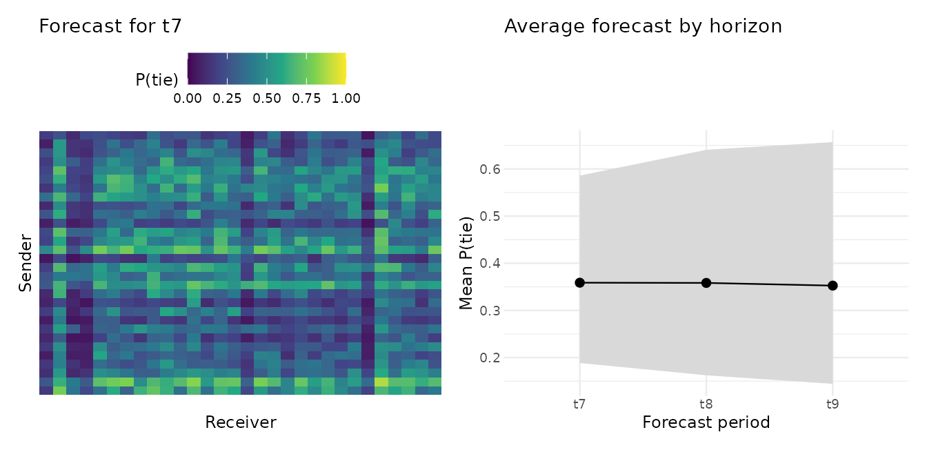

The heatmap shows the model does not forecast a uniform network: some sender/receiver pairs carry a much higher predicted tie probability than others, inherited from their estimated additive effects and the recovered trade coefficient. The horizon panel shows the average predicted probability staying roughly level (the coefficient is mean-reverting) while its credible band widens with h – the visual signature of accumulating forecast uncertainty.

The forecast propagates (β_t, a_t, b_t, U_t, V_t) forward by drawing from the joint posterior of the dynamic state-space hyperparameters (ρ_β, σ_β, ρ_ab, σ_ab, ρ_uv, σ_uv) for each posterior draw. The same forecasting machinery works for any family; the binary example above is just for illustration. For family = "normal", type = "response" returns the forecasted continuous outcome; for family = "poisson", the response-scale forecast multiplies exp(η) by the future-period exposure (pass via newexposure = ...; see the period_exposure section below).

Poisson exposure offsets via period_exposure

For family = "poisson", pass period_exposure = e to lame() (a non-negative numeric vector of length T) when the per-period rate should be scaled by a known exposure (e.g. weeks observed, population size, number of edge-formation opportunities). The sampler treats log(period_exposure[t]) as a fixed offset on the linear predictor: the Poisson mean for period t becomes period_exposure[t] * exp(η_t) instead of exp(η_t). Setting a non-trivial (any value not equal to 1) period_exposure for a non-Poisson family is rejected with an error. When you call predict(fit, h = K) later without newexposure, the response-scale forecast reuses the last observed exposure for every future period; pass newexposure = rep(e_new, K) to forecast under a different exposure path.

Step 3: Counterfactual forecasts

Pass newdata = list_of_h_future_X_arrays to combine alternative future covariates with the forecast. Each array is n x n x p and the slice order along the 3rd dimension must match the original dimnames(Xdyad[[1]])[[3]] from the fit (here a single slice, trade).

set.seed(1)   # forecast draws are stochastic; seed so the printed delta summary reproduces
# baseline scenario: freeze the trade covariate at the last observed period
last_X <- Xdyad[[length(Xdyad)]]
X_future <- list(last_X, last_X, last_X)
fc_cf <- predict(fit, h = 3, type = "response", newdata = X_future)

# counterfactual: shift every dyad's trade covariate up by one unit
# going forward. Because `trade` is a standardised (mean-zero) covariate,
# an additive +1 shift -- "one standard deviation more trade for every
# pair" -- is the interpretable counterfactual; a multiplicative scaling
# would be meaningless on a centred covariate (see caution 2 below).
X_future_up <- lapply(X_future, function(x) {
    x[, , 1] <- x[, , 1] + 1
    x
})
fc_up <- predict(fit, h = 3, type = "response", newdata = X_future_up)

# delta is the per-dyad change in posterior-mean cooperation probability
# at h = 3, attributable solely to the +1 trade shift
delta_h3 <- fc_up[[3]] - fc_cf[[3]]
summary(as.vector(delta_h3))
#>     Min.  1st Qu.   Median     Mean  3rd Qu.     Max. 
#> -0.03506  0.05346  0.09025  0.07910  0.11019  0.13151

The trade coefficient is positive and mean-reverting, so a one-unit increase in trade raises the posterior-mean cooperation probability at h = 3 on average (the mean and median of delta_h3 are both positive). The per-dyad shift varies in size, and a minority of dyads even show a small negative shift: the three-step-ahead forecast of the coefficient is itself uncertain (its posterior at h = 3 is centred well above zero but has nonzero mass below it), and the marginal probit effect $\phi(\eta)\,\beta$ is smallest for dyads whose baseline linear predictor $\eta = a_i + b_j + \beta x_{ij}$ already sits far from the 0.5 probability boundary. For substantive interpretation, summarise delta_h3 for the dyads that matter rather than reporting the aggregate summary().

Two cautions on counterfactual covariates. (1) Because dynamic_beta draws the coefficient path forward from its posterior, the same covariate change can produce different magnitudes at different horizons, because the multiplier on trade is itself uncertain and drifting. (2) Multiplicative counterfactuals on covariates that take negative or zero values (such as this centred trade covariate) do not make substantive sense; prefer additive shifts there, which is why we used + 1 rather than * 2 above.

Step 4: Visualise the coefficient path

library(ggplot2)
autoplot(fit, probs = c(0.025, 0.5, 0.975)) +
    labs(title = "Posterior coefficient paths",
         subtitle = "median + 95% interval",
         x = "Time period", y = "Coefficient value")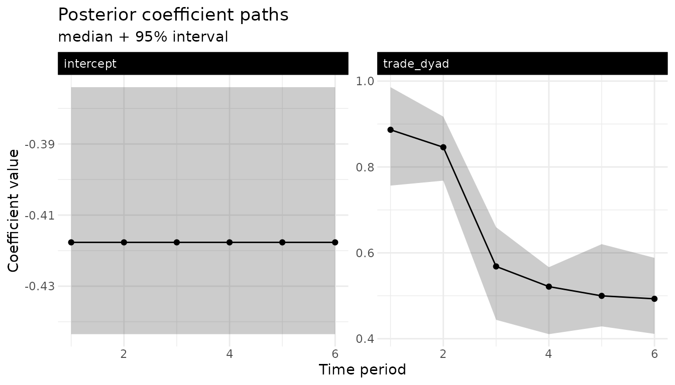

The ribbon shows the posterior 95% credible interval around the posterior median per coefficient and period; faceted by coefficient.

Step 5: Forecast diagnostics

predict(fit, h = ...) fires a one-per-fit warning if the upper 97.5% credible bound on ρ_β reaches 0.99 (i.e. the posterior puts non-trivial mass near the unit root). On the mean-reverting fit above that bound sits at 0.923, so the warning does not fire and the forecasts are well-posed. The two regimes still have qualitatively different forecast-variance behavior, and getting this distinction right matters for picking your horizon:

• AR(1), dynamic_beta_kind = "ar1" with $|\rho| < 1$: the conditional $h$-step variance of $\beta_{T+h}$ given the training window is $\sigma_\beta^2 \cdot (1 - \rho^{2h}) / (1 - \rho^2)$. It saturates (the increment from $h$ to $h+1$ shrinks geometrically to zero) and the limit is the stationary variance $\sigma_\beta^2 / (1 - \rho^2)$. That stationary level itself blows up as $\rho \to 1$, so AR(1) is still informative at long horizons only when $\rho$ is comfortably bounded away from 1.
• RW1, dynamic_beta_kind = "rw1": $\rho = 1$ by construction and the $h$-step variance is exactly $\sigma_\beta^2 \cdot h$, linear growth in $h$, never saturating.

In words: AR(1) eventually forgets the training window and falls back to a stationary distribution; RW1 keeps adding innovation variance every period. AR(1) forecasts can stay tight for moderate $h$ when $\rho$ is small; RW1 forecasts get linearly wider every step regardless. When the AR(1) stationarity warning fires and the underlying process is genuinely unit-root, refit with dynamic_beta_kind = "rw1"; if the AR(1) posterior on $\rho$ is near-but-not-at 1 and the science says “should mean-revert eventually,” stick with AR(1) but cap your reported horizon at $h \approx 3$. The warning printed by predict() states whichever of these two variance behaviours applies to your dynamic_beta_kind.

Watching it fail: a sparse, short, drifting panel

Everything above describes the failure mode; here it is actually happening. We simulate the kind of panel the Step 1 note warned about: fewer actors, only four periods, single-digit tie density in the early periods, and a covariate effect that drifts upward instead of mean-reverting. There is no long-run level for the AR(1) to find, so the posterior on $\rho_\beta$ runs up against the unit root:

set.seed(2026)
n_sp <- 20
T_sp <- 4
beta_drift <- c(0.4, 0.9, 1.4, 1.9)   # drifts up; never mean-reverts
X_sp <- lapply(seq_len(T_sp), function(t) {
    x <- matrix(rnorm(n_sp * n_sp), n_sp, n_sp)
    array(x, dim = c(n_sp, n_sp, 1),
          dimnames = list(NULL, NULL, "sanction_risk"))
})
Y_sp <- lapply(seq_len(T_sp), function(t) {
    eta <- -2 + beta_drift[t] * X_sp[[t]][, , 1]
    Yt  <- matrix(rbinom(n_sp * n_sp, 1, pnorm(eta)), n_sp, n_sp)
    diag(Yt) <- NA
    rownames(Yt) <- colnames(Yt) <- sprintf("s%02d", seq_len(n_sp))
    Yt
})
names(Y_sp) <- paste0("t", seq_len(T_sp))
sapply(Y_sp, function(y) round(mean(y, na.rm = TRUE), 3))  # sparse early on
#>    t1    t2    t3    t4 
#> 0.034 0.055 0.118 0.161

fit_sparse <- lame(
    Y_sp, Xdyad = X_sp,
    family = "binary", R = 0,
    dynamic_beta = "dyad", dynamic_beta_kind = "ar1",
    nscan = 400, burn = 100, odens = 5,
    verbose = FALSE
)
round(quantile(fit_sparse$RHO_BETA, c(0.5, 0.975)), 3)
#>   50% 97.5% 
#> 0.813 0.953

The upper 97.5% bound on $\rho_\beta$ is now 0.953 – past the 0.99 threshold – so the forecast call itself raises the warning:

set.seed(1)
fc_sparse <- predict(fit_sparse, h = 6, type = "response",
                     interval = "credible")

That is the diagnostic doing its job at forecast time. To see what the near-unit-root posterior does to the intervals, compare how the average 95% forecast-interval width grows with the horizon on this fit versus the mean-reverting Step 1 fit:

set.seed(1)
fc_healthy <- predict(fit, h = 6, type = "response",
                      interval = "credible")
width_by_h <- function(fc) {
    sapply(fc, function(m) mean(m$upper - m$lower, na.rm = TRUE))
}
w_healthy <- width_by_h(fc_healthy)
w_sparse  <- width_by_h(fc_sparse)
round(rbind(mean_reverting = w_healthy, near_unit_root = w_sparse), 3)
#>                 [,1]  [,2]  [,3]  [,4]  [,5]  [,6]
#> mean_reverting 0.313 0.401 0.458 0.500 0.526 0.496
#> near_unit_root 0.227 0.280 0.413 0.473 0.471 0.447

# at h = 3, how many of the dyads the covariate actually moves (top
# decile of |sanction_risk|) get an interval spanning nearly all of
# [0, 1]?
x_last <- X_sp[[T_sp]][, , 1]
hi_x   <- abs(x_last) >= quantile(abs(x_last), 0.9)
deg_h3 <- mean(fc_sparse[[3]]$lower[hi_x] < 0.05 &
               fc_sparse[[3]]$upper[hi_x] > 0.95, na.rm = TRUE)
round(deg_h3, 2)
#> [1] 0.52

width_df <- data.frame(
    h     = rep(seq_along(w_healthy), 2),
    fit   = rep(c("mean-reverting (Step 1 fit)",
                  "near-unit-root (sparse fit)"), each = length(w_healthy)),
    width = c(w_healthy, w_sparse)
)
ggplot(width_df, aes(h, width, linetype = fit)) +
    geom_line() + geom_point(size = 1.8) +
    labs(title = "Forecast interval width by horizon",
         x = "Forecast horizon h", y = "Mean 95% interval width") +
    theme_bw(base_size = 9) +
    theme(panel.border = element_blank(), axis.ticks = element_blank(),
          legend.position = "top", legend.title = element_blank())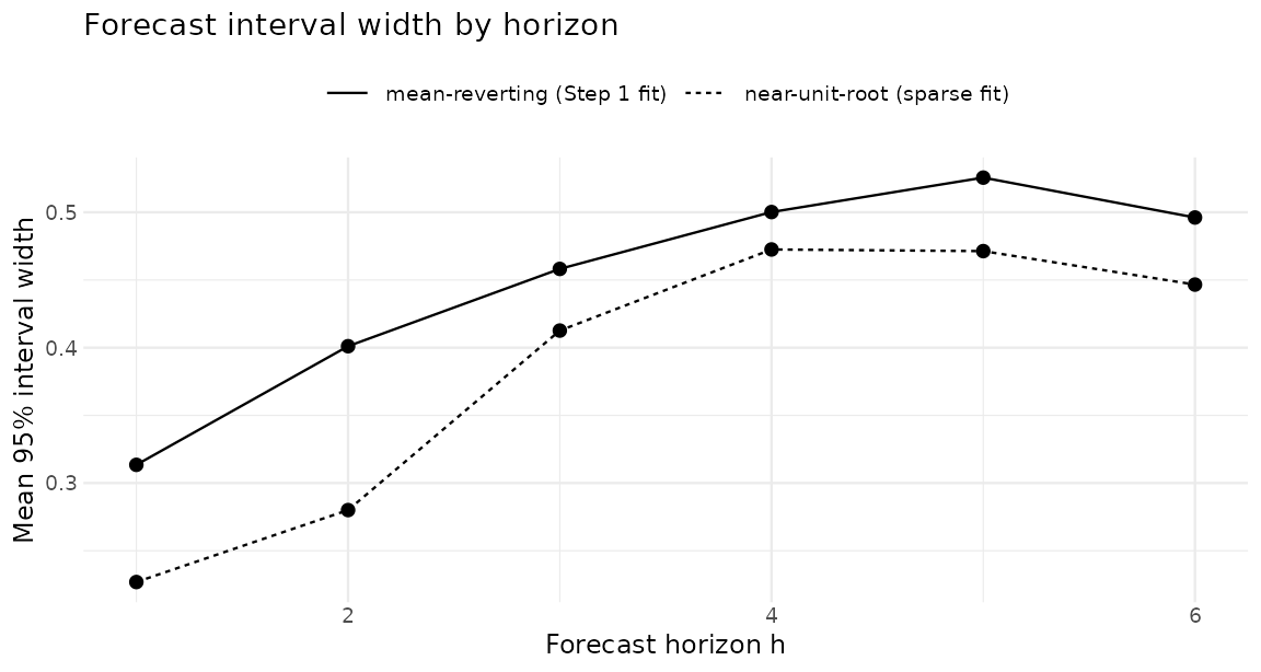

Read the growth, not the levels: the sparse fit’s absolute widths are smaller only because most of its predicted probabilities sit near zero (the network is sparse). The mean-reverting fit’s width grows by a factor of just 1.6 across the whole horizon and is flat from about h = 4 on – the saturation the AR(1) bullet above predicts. The near-unit-root fit’s width has grown by a factor of 2 by h = 6 and is still climbing – the growth you get when $\rho_\beta$ sits at the unit root, damped here only by the bounded [0, 1] probability scale. And the degeneracy lands exactly where it hurts: among the dyads the covariate actually moves (the top decile of |sanction_risk|), 52% of the h = 3 intervals already span essentially the whole unit interval, on a network whose observed density never exceeded 16%. A forecast interval of [0, 1] for a rare-event dyad says nothing at all – which is precisely what the warning is telling you. The remedy is the one stated above: refit with dynamic_beta_kind = "rw1" if the drift is real, and in either case do not report horizons past $h \approx 3$.

For a longer-horizon diagnostic, use the exact rolling-origin leave-future-out CV:

# refit on Y[1:(t-1)] for each t in periods and score Y[[t]].
# Skip the very first leave-out (would leave a 1-period training window
# which is too short for dynamic_beta); use the last 2 origins.
set.seed(1)  # the internal h=1 forecast draws inside lfo() are stochastic; seed for reproducibility
T_fit <- length(fit$YPM)
lfo_periods <- tail(seq_len(T_fit), max(1L, min(2L, T_fit - 2L)))
lfo_res <- lfo(fit, periods = lfo_periods, refit = TRUE,
               nscan = 100, burn = 25, odens = 5, verbose = FALSE)
print(lfo_res)
#> 
#> ── Exact rolling-origin LFO ──
#> 
#> Periods evaluated: 5 and 6
#> Refit per leave-out: TRUE
#> Total elpd_lfo: -1189.6
#>  period      elpd n_obs
#>       5 -621.6205   870
#>       6 -567.9607   870

The nscan = 100, burn = 25, odens = 5 settings inside lfo() are chosen so the vignette builds in well under a minute on a laptop. They give 100 / 5 = 20 stored draws per leave-out refit (burn-in is run and discarded, not subtracted from nscan), enough to return a sensible point estimate of per-period elpd for demonstration, but tighter than you should use when the LFO output drives an inference. For real analyses, pass nscan = 5000, burn = 1000, odens = 25 (or whatever matches your lame() baseline) and verify the per-period elpd is stable across two independent runs before relying on it.

On this mean-reverting fit the two leave-out folds return per-period elpd of roughly -560 to -620 over 870 scored dyads (about -0.65 to -0.7 nats/dyad), and the two folds are close to each other – the model forecasts the held-out period about as well at origin 5 as at origin 6, which is what you want to see when there is no late regime change. If elpd instead dropped sharply at the last fold, that would be the empirical signal of a regime change near the end of your training window; reach for detect_change_point(fit) (a heuristic Bayes-factor diagnostic) to localise it.

Probability-integral-transform (PIT) calibration

forecast_pit() complements lfo() by asking a sharper question: given the held-out outcomes, is the h-step posterior-predictive distribution itself well calibrated? For continuous families the PIT is the Gaussian CDF evaluated at the observation; for binary / Poisson / ordinal it is the Czado-Gneiting-Held randomised PIT (Czado, Gneiting & Held 2009). A well-calibrated forecast produces PIT values that are Uniform(0, 1).

# fit on the first five periods, hold out the sixth
fit_train <- lame(
    Y[1:5], Xdyad = Xdyad[1:5],
    family = "binary", R = 0,
    dynamic_beta = "dyad",
    nscan = 100, burn = 30, odens = 5,
    verbose = FALSE
)
set.seed(1)   # the randomised PIT draws are stochastic; seed for reproducibility
pit <- forecast_pit(fit_train, y_future = list(Y[[6]]))
print(pit)
#> 
#> ── Forecast PIT calibration check ──
#> 
#> • Family: "binary"
#> • Forecast horizon: 1
#> • Held-out dyads: 870
#> • KS stat vs Uniform(0,1): 0.018
#> • KS p-value: 0.941
#> • Fraction in [0.025, 0.975]: 0.946 (expect 0.95)
#> PIT values are consistent with Uniform(0, 1) at the 5% level.

plot(pit) renders the PIT values against the Uniform(0, 1) reference that a perfectly calibrated forecast would follow:

plot(pit)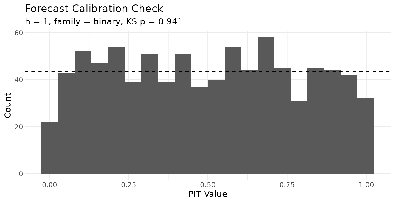

Bars that hug the uniform reference indicate a well-calibrated forecast. A U-shape (mass piling up in the tails) is the signature of an over-confident forecast whose intervals are too narrow; a central hump is the opposite, an under-confident forecast with intervals that are too wide. On this single binary held-out period the randomised PIT is noisy, so read the plot for gross departures rather than small wiggles, and corroborate it with cover_95 below.

(fit_train has only five periods to pin down $\rho_\beta$, so its posterior is wider than that of the six-period fit above; on very short or sparse panels that extra uncertainty can spill past the forecast-time unit-root threshold, exactly as the drifting sparse panel earlier in Step 5 demonstrated. Here it stays clear of the threshold – the unit-root warning does not fire for fit_train and the print(pit) output above is clean. If you do see that warning on your own shorter-window fit, read it as a caution about the training fit’s forecast variance rather than a defect in the PIT check – the calibration summaries below remain meaningful either way.)

Read the two summaries together. pit$cover_95 – the fraction of held-out cells whose observed outcome falls in the central 95% posterior-predictive interval, target 0.95 – is the stable summary; here it lands at about 0.94, close to nominal, so the forecast intervals have roughly the right width. pit$ks_p tests whether the full PIT distribution is Uniform(0, 1); a value below 0.05 flags mis-calibration. For a binary outcome the PIT is the randomised Czado-Gneiting-Held version, so on a single held-out period ks_p carries randomisation noise on top of ordinary sampling noise. Here it is 0.941 – above 0.05, so this run passes – but redrawing the randomisation alone can move that p-value from below 0.05 to far above it, so a single KS p-value on one held-out period neither confirms nor condemns the forecast. (We seed the chunk only so the printed value reproduces.) Treat cover_95 as the headline and ks_p as corroborating evidence. For a sharper test, hold out two or more periods and pair plot(pit) with pit$pit to see whether any mis-calibration is in the tails (over- vs under-dispersion) or the centre (location bias). On a sparse, short, near-unit-root panel both summaries degrade together – cover_95 drops well below 0.95 and ks_p collapses toward 0 – the calibration-side signature of the forecast-variance explosion the Step 5 warning flags.

Comparing two fits with loo_compare()

When you have two candidate specifications, say a static-beta baseline and a dynamic_beta = "dyad" variant, loo::loo_compare() is the one-liner that ranks them on out-of-sample predictive performance. Both fits need save_log_lik = TRUE so loo() can read the stored pointwise log-likelihood matrix off fit$log_lik:

# run this after fitting both candidates with converged chains
fit_static <- lame(
    Y, Xdyad = Xdyad, family = "binary", R = 0,
    nscan = 5000, burn = 1000, odens = 25,
    save_log_lik = TRUE,
    verbose = FALSE
)
fit_dyn <- lame(
    Y, Xdyad = Xdyad, family = "binary", R = 0,
    dynamic_beta = "dyad",
    nscan = 5000, burn = 1000, odens = 25,
    save_log_lik = TRUE,
    verbose = FALSE
)

# rank the two fits: the row with elpd_diff = 0 is the best,
# subsequent rows show elpd_diff and its SE relative to it. Pass a NAMED
# list so the rows are labelled by model name rather than "model1"/"model2".
cmp <- loo::loo_compare(list(fit_static = loo::loo(fit_static),
                             fit_dyn    = loo::loo(fit_dyn)))
cmp

best     <- rownames(cmp)[1]
runnerup <- rownames(cmp)[2]
diff_val <- abs(round(cmp[2, "elpd_diff"], 1))
se_val   <- round(cmp[2, "se_diff"], 1)
ratio    <- round(diff_val / se_val, 1)

How to read this output. The top row is the preferred model and has elpd_diff = 0. Each subsequent row gives the difference in expected log pointwise predictive density relative to that model and the standard error of the difference. A difference that is large relative to its standard error supports the preferred model; when the two are similar, the specifications are not distinguishable on this predictive criterion. Read the Pareto-$k$ diagnostics before interpreting the ranking.

Because family = "binary" is one of the five families with an exact closed-form log-likelihood (normal, binary, cbin, poisson, ordinal; see the log-lik scale discussion in the Dynamic Effects vignette), the two elpd_loo values here are on the response scale and the absolute numbers are directly comparable to a loo() result from a probit-link brms fit on the same data, modulo the lame Gibbs sampler’s R-hat / ESS being satisfactory. For the rank likelihood frn, the default observed_exact falls back to an augmented-Z normal approximation and is only valid for relative comparison within lame; opt in to log_lik_method = "observed_ghk" for the exact marginal on that family.

Memory-conscious long runs

If the in-memory log-likelihood matrix from save_log_lik = TRUE would exceed RAM, pass save_log_lik = "chunked" instead. The on-disk chunks are recovered transparently by loo(), or can be read back directly as a matrix with read_log_lik(fit):

fit_chk <- lame(
    Y, Xdyad = Xdyad, family = "binary", R = 0,
    dynamic_beta = "dyad",
    nscan = 2000, burn = 500, odens = 5,
    save_log_lik = "chunked",          # per-column-chunk binary files
    log_lik_chunk_size = 5000L,
    verbose = FALSE
)
loo::loo(fit_chk)                       # reads the chunks transparently

See also

• vignettes/dynamic_effects.Rmd: the full reference on dynamic_beta / dynamic_ab / dynamic_uv and the decision tree for picking dynamic_beta_kind.
• ?predict.lame: argument reference for h, newdata, type, by_draw.
• ?autoplot.lame: ggplot ribbon plot for dynamic coefficients.
• ?lfo: exact rolling-origin LFO CV.