Your First AME Model

Cassy Dorff, Shahryar Minhas, and Tosin Salau

2026-07-25

Why Network Models?

Imagine you’re studying friendships in a high school. You have data on who nominated whom as a friend, plus information about each student (gender, race, grade). A natural first instinct is to run a logistic regression: does sharing the same gender predict friendship?

The problem is that friendships aren’t independent observations. Some students are more social (they nominate lots of friends), some are more popular (they receive lots of nominations), and friendships tend to be reciprocated: if Alice names Bob, Bob is more likely to name Alice. A standard regression ignores all of this, and your standard errors will be wrong.

The Additive and Multiplicative Effects (AME) model handles these dependencies directly. It gives each actor a sender effect ($a_i$, how social they are), a receiver effect ($b_j$, how popular they are), and a position in a latent space ($u_i$, $v_j$) that captures who tends to connect with whom beyond what the covariates explain. The additive effects enter as $a_i + b_j$; the latent positions enter multiplicatively as the dot product $u_i'v_j$. Think of it as a regression that takes network structure seriously.

The Data

We’ll analyze a friendship network from the Add Health study, a longitudinal study of adolescents in the United States. The addhealthc3 dataset in lame contains a directed friendship nomination network along with student characteristics.

library(lame)
library(ggplot2)
set.seed(6886)

# load the Add Health friendship network
data(addhealthc3)

# convert valued network to binary (any nomination = friendship)
Y <- (addhealthc3$Y > 0) * 1
X_nodes <- addhealthc3$X

n <- nrow(Y)
cat("Students:", n, "\n")
#> Students: 32
cat("Friendships:", sum(Y, na.rm = TRUE), "\n")
#> Friendships: 127
cat("Network density:", round(mean(Y, na.rm = TRUE), 3), "\n")
#> Network density: 0.128

Notice the na.rm = TRUE calls: network data often has missing entries (the diagonal is NA because self-ties are undefined). The model handles missing values internally via data augmentation, so NAs can stay in the matrix – including dyads built from missing covariates (here race and grade have a handful), which ame() likewise treats as unobserved.

Before modeling: how much do students vary in their number of friends?

out_degree <- rowSums(Y, na.rm = TRUE)
in_degree <- colSums(Y, na.rm = TRUE)

degree_df <- data.frame(
    Degree = c(out_degree, in_degree),
    Type = rep(c("Nominations sent", "Nominations received"), each = n)
)

ggplot(degree_df, aes(x = Degree)) +
    geom_histogram(binwidth = 1) +
    facet_wrap(~Type, ncol = 2) +
    labs(x = "Number of Ties", y = "Count") +
    theme_bw() +
    theme(
        panel.border = element_blank(),
        axis.ticks = element_blank(),
        legend.position = "top",
        strip.background = element_rect(fill = "black", color = "black"),
        strip.text = element_text(color = "white", hjust = 0)
    )

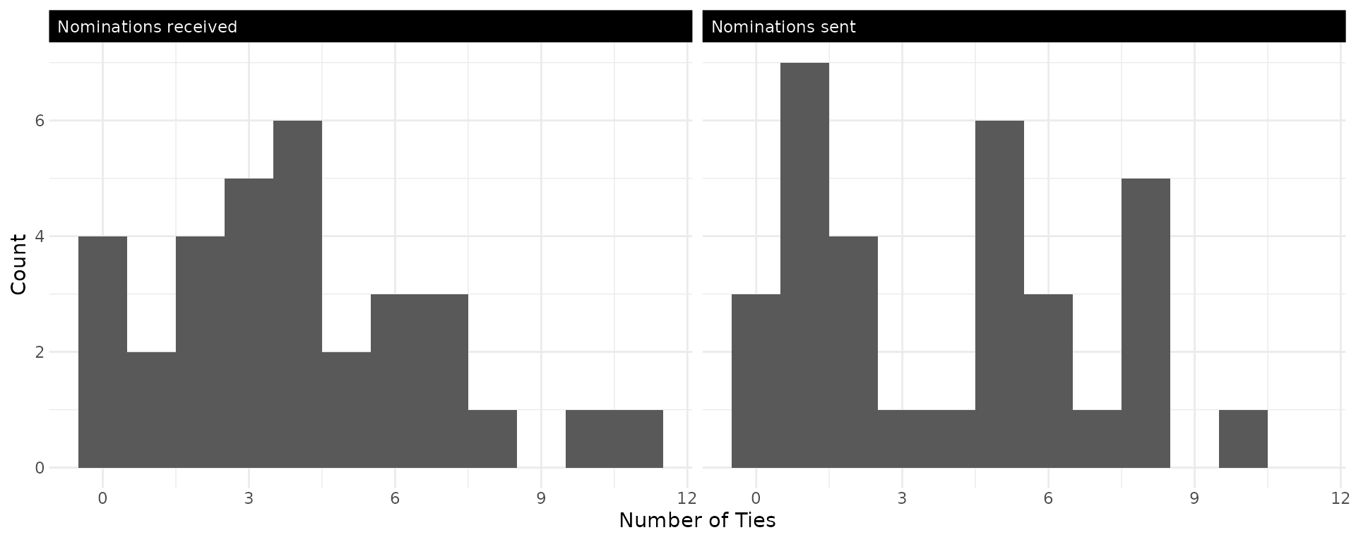
Some students are much more social than others, and some much more popular – exactly what the sender and receiver random effects will capture.

Building Covariates

The classic question in friendship networks is homophily: do birds of a feather flock together? We’ll test whether students are more likely to be friends with others of the same gender, race, and grade.

We deliberately include both same_grade (binary) and grade_diff (continuous: grades apart) to illustrate a common modeling pitfall, collinearity: they measure nearly the same thing, and we’ll see the consequences in the results below.

# `outer(x, x, FUN)` builds an n x n matrix whose (i,j) entry is FUN(x[i], x[j]).
# So `outer(female, female, "==")` returns TRUE where students i and j share the
# same gender. Multiplying by 1 converts TRUE/FALSE to 1/0.
#
# homophily indicators: 1 if same, 0 if different
same_female <- outer(X_nodes[,"female"], X_nodes[,"female"], "==") * 1
same_race <- outer(X_nodes[,"race"], X_nodes[,"race"], "==") * 1
same_grade <- outer(X_nodes[,"grade"], X_nodes[,"grade"], "==") * 1
# absolute grade difference; same shape, but a continuous covariate
grade_diff <- abs(outer(X_nodes[,"grade"], X_nodes[,"grade"], "-"))

# pack into a 3D array (n x n x p)
Xdyad <- array(NA, dim = c(n, n, 4))
Xdyad[,,1] <- same_female
Xdyad[,,2] <- same_race
Xdyad[,,3] <- same_grade
Xdyad[,,4] <- grade_diff
dimnames(Xdyad)[[3]] <- c('same_female', 'same_race', 'same_grade', 'grade_diff')
for(k in 1:4) diag(Xdyad[,,k]) <- NA

# nodal covariates (sender and receiver characteristics)
Xrow <- X_nodes[, c("female", "grade")]
Xcol <- X_nodes[, c("female", "grade")]

Fitting the Model

Now the fun part. We fit a binary probit AME model with:

• Covariates for homophily effects
• Sender and receiver random effects (sociality / popularity)
• Dyadic correlation (reciprocity)
• 2-dimensional latent space (residual clustering)

A note for ERGM users: what AME assumes

If you’re coming from ergm / statnet, the key difference is the dependence assumption. ERGM uses change statistics (e.g. gwesp, triangle, kstar) to encode unconditional higher-order dependence: changing one tie shifts the probability of other ties directly. AME instead assumes conditional dyadic independence: given the additive effects $(a_i, b_j)$, the latent positions $(u_i, v_j)$, the dyadic correlation $\rho$, and the covariates, all dyads are independent, and higher-order structure is captured indirectly by integrating over the latent effects.

Three practical consequences:

• No degeneracy. AME avoids the model-degeneracy failure modes of ERGMs with triangle or unconstrained kstar terms.
• No change-statistic interpretation of $\beta$. A coefficient on same_grade is a partial association on the probit-latent scale, not a log-odds change conditional on the rest of the network.
• Some triangle structure is missed. When transitive closure is the substantive target (gwesp is the leading example), ERGM is the right tool; for structural pattern + actor heterogeneity + covariate effects with calibrated uncertainty, AME is generally the more stable estimator.

fit <- ame(Y,
                    Xdyad = Xdyad,
                    Xrow = Xrow,
                    Xcol = Xcol,
                    R = 2,              # 2D latent space
                    family = "binary",  # probit model for 0/1 data
                    rvar = TRUE,        # sender random effects
                    cvar = TRUE,        # receiver random effects
                    dcor = TRUE,        # dyadic correlation (reciprocity)
                    burn = 100,         # compact burn-in for this worked example
                    nscan = 500,        # compact post-burn-in run for the vignette
                    odens = 25,         # thinning
                    verbose = FALSE,
                    gof = TRUE)

What Did We Find?

summary(fit)
#> 
#> === AME Model Summary ===
#> 
#> Call:
#> [1] "Y ~ intercept + dyad(same_female, same_race, same_grade, grade_diff) + row(female, grade) + col(female, grade) + a[i] + b[j] + rho*e[ji] + U[i,1:2] %*% V[j,1:2], family = 'binary'"
#> 
#> Regression coefficients:
#> ------------------------
#>                  Estimate StdError z_value p_value CI_lower CI_upper    
#> intercept          -3.947    1.092  -3.614       0   -5.955   -2.142 ***
#> female_row         -0.535    0.385  -1.388   0.165   -1.208    0.033    
#> grade_row           0.064    0.071   0.902   0.367   -0.056    0.197    
#> female_col         -0.427    0.241  -1.771   0.077   -0.863   -0.115   .
#> grade_col           0.308    0.075   4.124       0     0.19    0.428 ***
#> same_female_dyad    0.229    0.223   1.028   0.304   -0.222    0.608    
#> same_race_dyad      0.089    0.265   0.336   0.737   -0.325     0.51    
#> same_grade_dyad     0.178    0.245   0.725   0.468   -0.183    0.618    
#> grade_diff_dyad    -0.711    0.095  -7.449       0   -0.922   -0.592 ***
#> ---
#> Signif. codes: 0 '***' 0.001 '**' 0.01 '*' 0.05 '.' 0.1 ' ' 1
#> Note: stars are a visual hint from posterior mean / SD only; for inference use the credible intervals.
#> 
#> Variance components:
#> -------------------
#>     Estimate StdError
#> va     0.459    0.200
#> cab    0.055    0.098
#> vb     0.244    0.075
#> rho    0.729    0.190
#> ve     1.000    0.000
#>   (va = sender, cab = sender-receiver covariance, vb = receiver,
#>    rho = dyadic correlation, ve = residual variance)

Let’s unpack the key results:

Homophily effects. The grade_diff coefficient is strongly negative and its credible interval excludes zero: students further apart in grade are much less likely to be friends. The same_female coefficient is positive (gender homophily) but its 95% credible interval includes zero – read the sign as suggestive, not the effect as established. The same_race coefficient captures race homophily after controlling for grade and gender.

The collinearity pitfall. same_grade and grade_diff measure nearly the same thing – a grade difference of 0 is the same-grade event – so the model cannot cleanly split the grade signal between them. It still identifies the dominant effect: grade_diff is strongly negative and stable from run to run (about -0.71, never near zero). What suffers is the partition: same_grade is left to absorb a small, noisy residual bump on top of the linear grade-distance trend. The lesson is about interpretation, not estimate instability: include one or the other, not both, so the grade effect lands on a single, clean coefficient.

Variance components. The sender variance (va) and receiver variance (vb) quantify how much students differ in sociality and popularity. The dyadic correlation (rho) captures reciprocity: values near 1 mean that if A nominates B, B almost always nominates A back. Reciprocity is strong here.

For binary networks with a probit link, the coefficients are on the latent scale, and the textbook “$0.4 \times \beta$” rule for converting them to probability changes is only sharp when the baseline probability is near 0.5 – which this sparse network is not. Rather than juggling correction factors, compute the quantity you actually want with predict(fit, type = "response") and contrast predicted probabilities under counterfactual covariate settings.

Did the Sampler Converge?

The model is estimated via MCMC (Markov chain Monte Carlo), so trace plots are the first check that the sampler explored the posterior thoroughly.

trace_plot(fit, params = "beta", ncol = 3)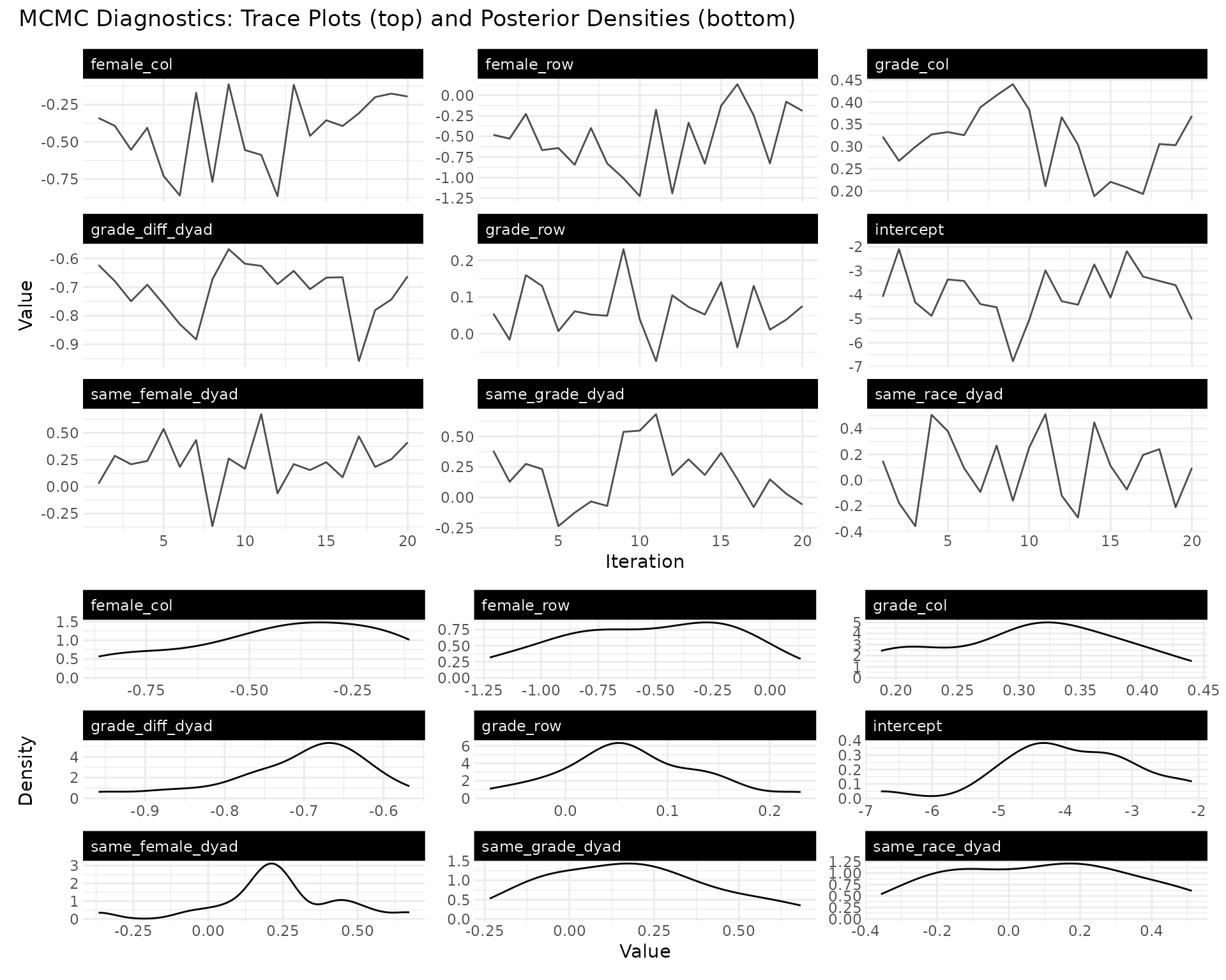

The regression coefficients are not the whole story, though – the slowest-mixing term in these fits is usually the dyadic correlation rho, so it deserves its own trace:

trace_plot(fit, params = "variance", include = "Dyadic Correlation")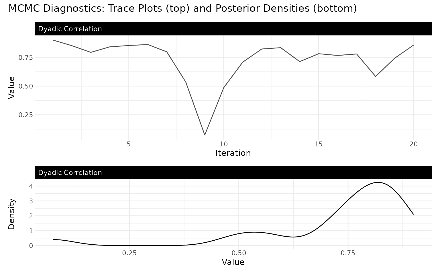

What to look for: Traces should fluctuate around a stable mean (long trends mean non-convergence) and densities should be smooth and unimodal. This fit stores 20 post-burn-in draws, enough to illustrate the workflow but not to establish convergence. rho, the reciprocity parameter, is often slower to mix than regression coefficients, so inspect it directly and use independent chains before drawing uncertainty statements from it.

Numerical convergence diagnostics: posterior::as_draws()

A trace plot is a sanity check, not a diagnostic. The Stan-era summary triple is split-$\hat R$, bulk ESS, and tail ESS; lame registers an as_draws() method, so the same posterior-package workflow you would run on a stanfit works here:

library(posterior)
draws <- posterior::as_draws(fit)              # draws_array [iter, chain, var]
posterior::summarise_draws(draws)              # mean, sd, q5, q95, rhat,
#> # A tibble: 14 × 10
#>    variable           mean  median     sd    mad      q5     q95   rhat ess_bulk
#>    <chr>             <dbl>   <dbl>  <dbl>  <dbl>   <dbl>   <dbl>  <dbl>    <dbl>
#>  1 intercept       -3.95   -4.10   1.09   1.05   -5.14   -2.18    1.03     13.2 
#>  2 female_row      -0.535  -0.503  0.385  0.480  -1.19   -0.0679  1.17      5.74
#>  3 grade_row        0.0644  0.0540 0.0713 0.0659 -0.0386  0.163   0.966    26.0 
#>  4 female_col      -0.427  -0.393  0.241  0.288  -0.861  -0.117   0.967    26.0 
#>  5 grade_col        0.308   0.314  0.0748 0.0793  0.193   0.417   1.32      3.64
#>  6 same_female_dy…  0.229   0.218  0.223  0.0979 -0.0771  0.543   0.954    26.0 
#>  7 same_race_dyad   0.0888  0.103  0.265  0.309  -0.293   0.507   0.961    26.0 
#>  8 same_grade_dyad  0.178   0.166  0.245  0.295  -0.130   0.554   1.05     15.2 
#>  9 grade_diff_dyad -0.711  -0.684  0.0954 0.0869 -0.886  -0.616   0.975    13.4 
#> 10 va               0.459   0.374  0.200  0.115   0.276   0.814   0.997    15.7 
#> 11 cab              0.0549  0.0643 0.0976 0.0916 -0.0765  0.187   1.58      2.81
#> 12 vb               0.244   0.229  0.0748 0.0577  0.163   0.379   1.01     16.0 
#> 13 rho              0.729   0.787  0.190  0.0959  0.465   0.863   1.02     11.7 
#> 14 ve               1       1      0      0       1       1      NA        NA   
#> # ℹ 1 more variable: ess_tail <dbl>
                                               # ess_bulk, ess_tail per param

The conventional thresholds are split-$\hat R$ < 1.01 for every monitored parameter and ess_bulk and ess_tail $\ge$ 400 per chain. This demonstration has only 20 draws from one chain, so it is not a convergence assessment. Within-chain split-$\hat R$ can flag a drifting chain, but it cannot reveal independent chains that settle in different parts of the posterior. One row will look degenerate in this table: ve is the latent residual variance, fixed at 1 for probit identification, so its draws are constant and posterior correctly reports NA for $\hat R$ and ESS.

Between-chain $\hat R$: ame_parallel(n_chains = 4)

For real convergence assessment, run four chains from different seeds and let summarise_draws() compute Rhat across chains:

# run this with four chains and longer runs for a convergence assessment
fit_mc <- ame_parallel(
    Y, Xdyad = Xdyad, Xrow = Xrow, Xcol = Xcol,
    family = "binary", R = 2,
    burn = 1000, nscan = 5000, odens = 25,
    n_chains = 4, cores = 4,            # use available cores when running locally
    combine_method = "pool",            # pooled fit retains chain identity
    verbose = FALSE
)
posterior::summarise_draws(posterior::as_draws(fit_mc))

Independent chains provide the comparison a single-chain summary cannot. Read the resulting split-$\hat R$, bulk ESS, and tail ESS together. If a parameter such as rho remains above the $\hat R$ threshold or has a low ESS, increase the run length and inspect its traces before using its posterior interval.

The pooled object carries a chain_indicator so as_draws() keeps chain identity separate; the same reshape feeds bayesplot::mcmc_trace() and tidybayes::tidy_draws() directly.

Other quick checks

Two cheap diagnostics worth running once per fit. lame is a Gibbs / Metropolis-Hastings sampler, not HMC, so it has no divergences – the closest analog is the per-block failure count exposed as fit$mh_counters; treat any block with more than 5% failures as suspicious. And prior_summary(fit) prints the hyperparameters actually used (defaults filled in), the cheapest way to catch a typo in a prior = list(...) override.

str(fit$mh_counters)
#> List of 5
#>  $ beta: int 0
#>  $ Sab : int 0
#>  $ s2  : int 0
#>  $ rho : int 0
#>  $ UV  : int 0

prior_summary(fit)
#> 
#> ── Priors in effect (ame fit) ──
#> 
#> Regression coefficients: `beta ~ N(0, g * sigma^2 * (X'X)^-1)` (g-prior).
#> `g` (top-level argument) = 992
#> Note: `g` is set at top level on `ame()` -- not inside `prior = list(...)`.
#> `Sab0` = "matrix(0.2032, 0, 0, 0.2032)"
#> `eta0` = "8"
#> `Suv0` = "matrix(0.2032, 0, 0, 0, 0, 0.2032, 0, 0, 0, 0, 0.2032, 0, 0, 0, 0,
#> 0.2032)"
#> `kappa0` = "13"

Model comparison: loo() and loo_compare()

If you refit with save_log_lik = TRUE, the fit carries a [n_stored, n_obs] pointwise log-likelihood matrix and loo::loo(fit) works directly via the registered S3 method:

# run this after fitting both candidates with converged chains
fit_ll <- ame(Y, Xdyad = Xdyad, Xrow = Xrow, Xcol = Xcol,
              family = "binary", R = 2,
              burn = 1000, nscan = 5000, odens = 25,
              save_log_lik = TRUE, verbose = FALSE)

# alternative model: drop the dyadic covariate
fit_ll_null <- ame(Y, Xrow = Xrow, Xcol = Xcol,
                   family = "binary", R = 2,
                   burn = 1000, nscan = 5000, odens = 25,
                   save_log_lik = TRUE, verbose = FALSE)

loo_dyad <- loo::loo(fit_ll)
loo_null <- loo::loo(fit_ll_null)

loo_dyad   # read the Pareto-k table before any elpd number

loo::loo_compare(list(with_dyad = loo_dyad, no_dyad = loo_null))

Start with the Pareto-$k$ table before reading elpd_diff. In an AME model, each dyad shares actor-level random effects ($a_i$, $b_j$, $u_i'v_j$) with many others, so leaving one dyad out can produce heavy-tailed importance weights. When many observations have large Pareto-$k$ values, use a held-out dyad evaluation or $K$-fold cross-validation rather than treating the PSIS-LOO ranking as decisive.

For the normal, binary, cbin, poisson, and ordinal families the stored log-likelihood is the exact family-specific Y density, so elpd_loo is directly comparable to a loo() from a brms or rstanarm fit to the same family; see ?loo.ame for the frn rank-likelihood caveat and fit$log_lik_method.

Does the Model Fit the Data?

Goodness-of-fit (GOF) checks whether the model can reproduce structural features of the observed network – degree heterogeneity, reciprocity, clustering – beyond dyad-level prediction.

gof_plot(fit)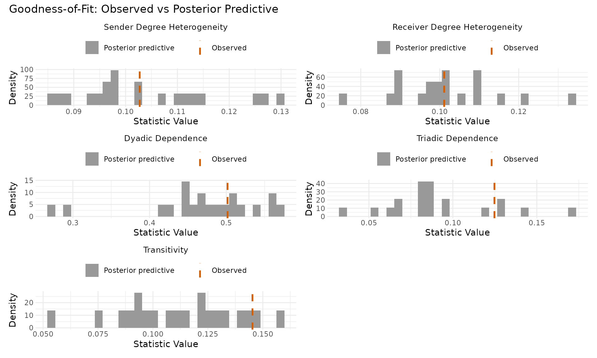

In each panel the grey histogram is the posterior-predictive distribution from networks simulated out of the fitted model, and the dashed orange vertical line is the observed value (colour and linetype dual-encode the contrast so it survives grayscale printing and colour-blind viewing). See ?gof_plot for the statistics = ... aliases and the exact column names stored in fit$GOF.

The observed values for Sender and Receiver Degree Heterogeneity and for Dyadic Dependence (essentially empirical reciprocity) fall inside their posterior-predictive histograms – those three features are explicitly modeled by the random effects, the variance components, and $\rho$. The two triad-level statistics tell a different story: observed Triadic Dependence sits toward the upper end of its histogram, and observed Transitivity in the upper tail. AME under-predicts triangle closure on this network, the expected signature of conditional dyadic independence: the latent space soaks up some triangle structure through clustering of the $u_i$, but there is no explicit closure term. If transitivity is your substantive target, fit an ERGM; if it is a diagnostic concern only, increasing R sometimes helps modestly.

You can also compute GOF after the fact using the gof() function, which accepts custom statistics. The built-in trans.dep panel is a correlation-style clustering measure; ERGM users will typically want the raw clustering coefficient (sna::gtrans, the scalar summary that gwesp(decay = 0, fixed = TRUE) targets), which takes a few lines as a custom stat:

# classic clustering coefficient: transitive triples / two-paths
trans_ratio <- function(Y) {
    Yb <- Y; Yb[is.na(Yb)] <- 0            # NA -> 0 for matrix multiply
    YY <- Yb %*% Yb
    triangles <- sum(YY * Yb)              # transitive triples
    two_path  <- sum(YY) - sum(diag(YY))   # two-paths (potential triangles)
    c(trans_ratio = triangles / max(two_path, 1))
}

gof_custom <- gof(fit, custom_gof = trans_ratio, nsim = 50, verbose = FALSE)
obs <- gof_custom[1, "trans_ratio"]
sim <- gof_custom[-1, "trans_ratio"]

# posterior-predictive p-value (right tail): near 0 = under-predicted
c(observed = round(obs, 3), sim_mean = round(mean(sim), 3),
  pp_p_right = round(mean(sim >= obs), 3))
#>   observed   sim_mean pp_p_right 
#>      0.485      0.410      0.053

Read this the way you would read ergm::gof(): pp_p_right is the fraction of simulated networks at or above the observed value, so a value near 0 means the model under-predicts the statistic. On Add Health it comes back at 0.105 (only two of the simulated networks reach the observed ratio in this short run) – the model produces triangles, but rarely concentrates them per two-path the way the data do, the same structural gap the built-in panels showed. See ?gof for adding further custom statistics (raw triangle counts, degree assortativity, and so on).

Visualizing the Latent Space

The multiplicative effects ($u_i'v_j$) place each student in a 2D latent space: students near each other in sender space (triangles) nominate similar friends, and students near each other in receiver space (circles) are nominated by similar students. Clusters likely share some unobserved characteristic (same social group, same extracurriculars) that drives friendship choices beyond gender, race, and grade.

uv_plot(fit, layout = "biplot", show.edges = FALSE, label.nodes = FALSE)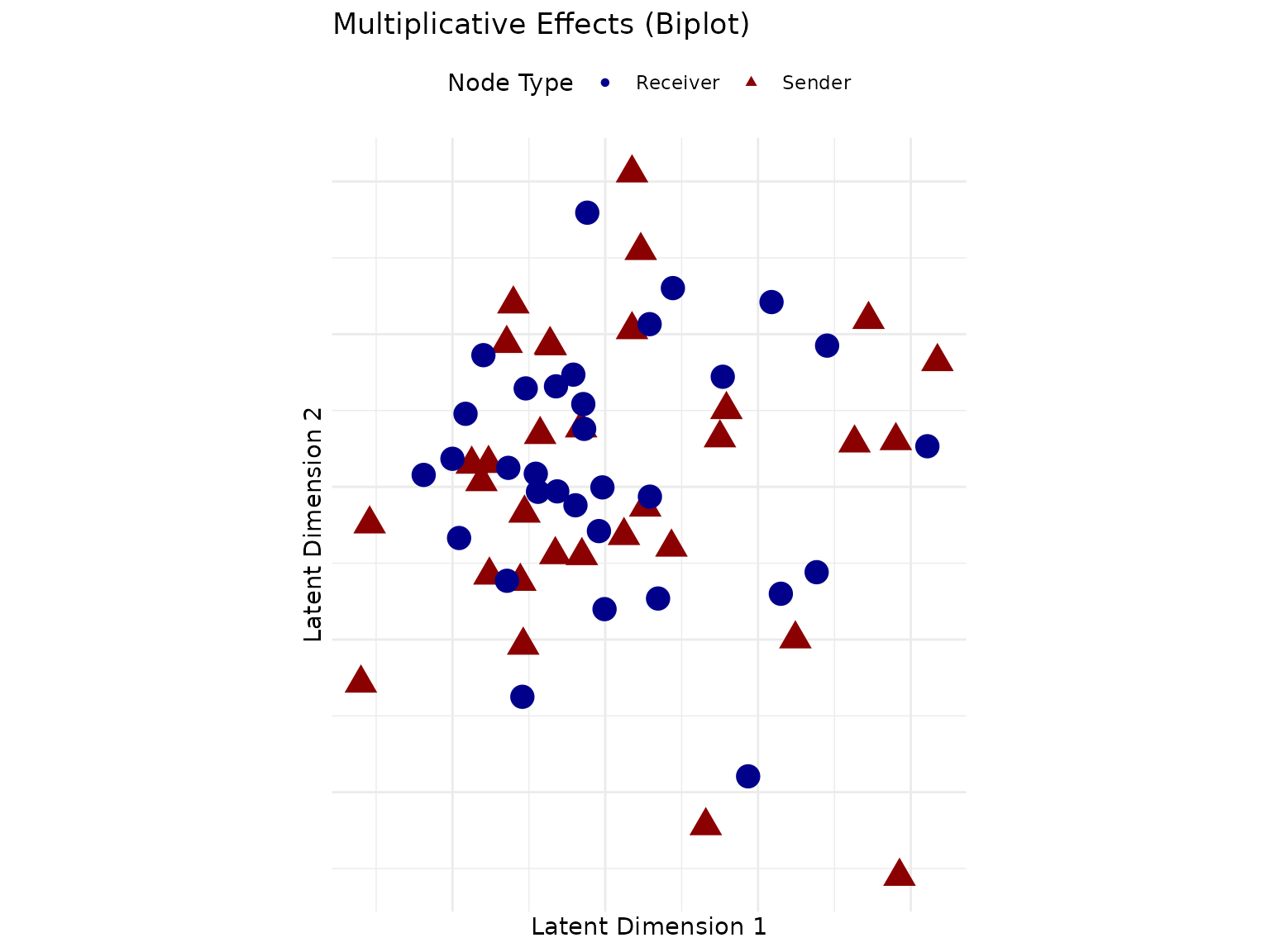

Who Are the Most Social / Popular Students?

The additive effects decompose individual heterogeneity into sender effects (sociality) and receiver effects (popularity):

p1 <- ab_plot(fit, effect = "sender", sorted = TRUE,
                            title = "Sender Effects (Sociality)")
p2 <- ab_plot(fit, effect = "receiver", sorted = TRUE,
                            title = "Receiver Effects (Popularity)")

library(patchwork)
p1 / p2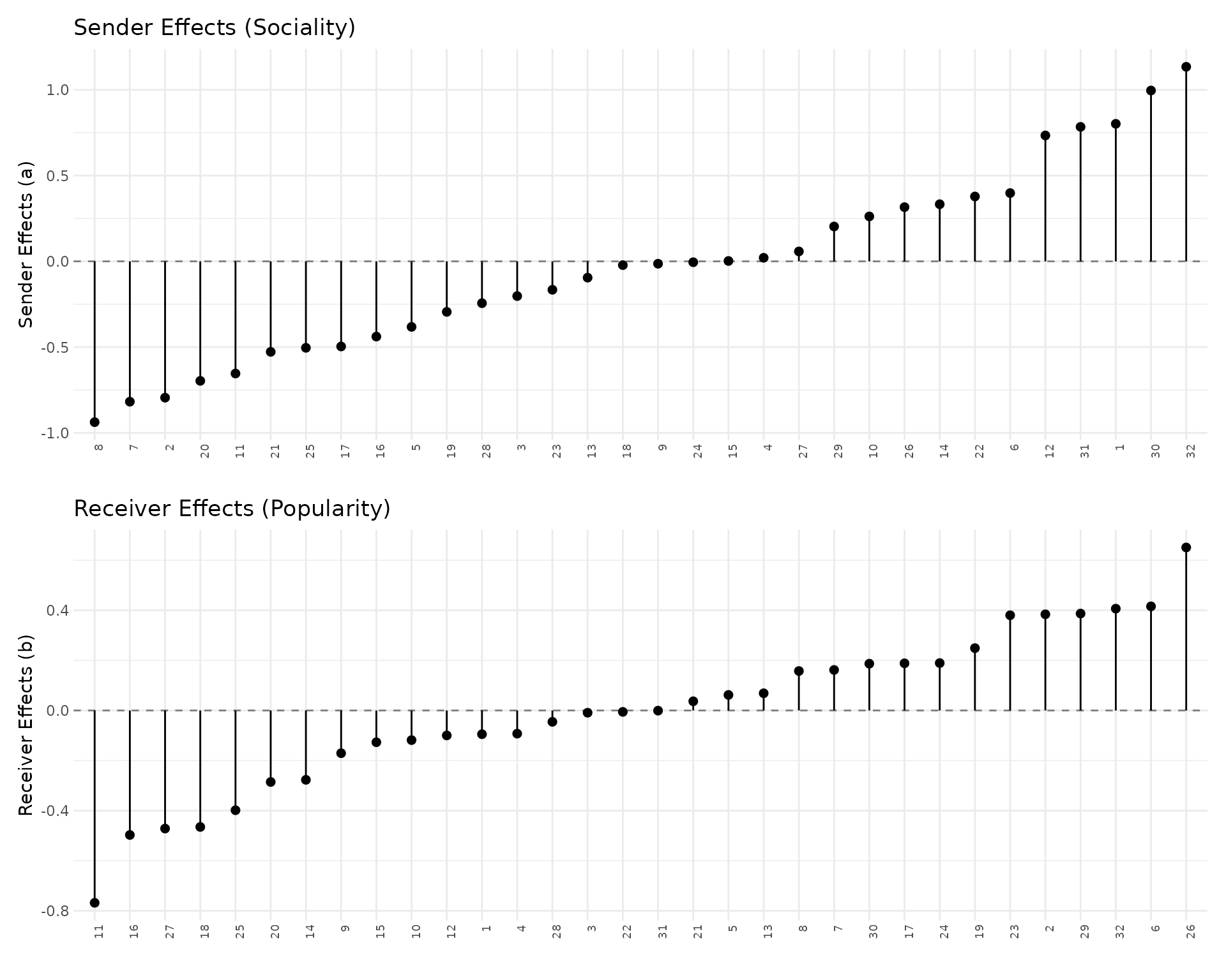

Students with large positive sender effects nominate more friends than expected given their covariates; those with large positive receiver effects receive more nominations.

Making Predictions

The model gives you predicted probabilities for every possible tie, useful for link prediction and for understanding dyad-level fit. One caution for sparse networks: predicting “no tie” for every dyad already gets most predictions right, so raw accuracy flatters the model – judge it against the modal-class baseline.

pred_resp <- predict(fit, type = "response")

# how well does the model classify?
Y_vec <- as.vector(Y)
pred_vec <- as.vector(pred_resp)
keep <- !is.na(Y_vec)

# simple classification at threshold 0.5
pred_binary <- (pred_vec[keep] > 0.5) * 1
confusion <- table(Actual = Y_vec[keep], Predicted = pred_binary)
knitr::kable(confusion, caption = "Confusion Matrix (threshold = 0.5)")

Confusion Matrix (threshold = 0.5)

	0	1
0	855	10
1	76	51

accuracy <- sum(diag(confusion)) / sum(confusion)
baseline <- max(mean(Y_vec[keep]), 1 - mean(Y_vec[keep]))  # always-predict-modal-class
cat("\nAccuracy:", round(accuracy, 3),
    " | Baseline (predict modal class):", round(baseline, 3),
    " | Lift:", round(accuracy - baseline, 3), "\n")
#> 
#> Accuracy: 0.913  | Baseline (predict modal class): 0.872  | Lift: 0.041

At density ~13% the modal-class baseline is ~0.87, so the relevant question is whether the model’s accuracy is materially above 0.87, not whether it crosses 0.5.

For link prediction, AUC-style metrics evaluate the model’s ability to rank true ties above non-ties across all thresholds. For sparse networks PR-AUC is the more informative summary: a model that always predicts “no tie” already has AUROC near 0.5 but PR-AUC near the network density, so the gap between PR-AUC and density is the metric of substantive interest.

# pROC: ROC curve and AUROC
# install.packages("pROC")
roc_obj <- pROC::roc(response = Y_vec[keep], predictor = pred_vec[keep],
                     quiet = TRUE)
auroc   <- as.numeric(pROC::auc(roc_obj))

# precrec: both ROC and Precision-Recall AUCs (the latter is more
# informative when the positive class is rare, as in friendship networks)
# install.packages("precrec")
ev <- precrec::evalmod(scores = pred_vec[keep], labels = Y_vec[keep])
precrec::auc(ev)   # returns AUROC and PR-AUC side-by-side
#>   modnames dsids curvetypes      aucs
#> 1       m1     1        ROC 0.9082017
#> 2       m1     1        PRC 0.7081509

cat("AUROC:", round(auroc, 3), "\n",
    "Baseline AUROC (random ranker):", 0.5, "\n",
    "Baseline PR-AUC (density of Y):", round(mean(Y_vec[keep]), 3), "\n")
#> AUROC: 0.908 
#>  Baseline AUROC (random ranker): 0.5 
#>  Baseline PR-AUC (density of Y): 0.128

Here that gap is wide: PR-AUC 0.719 against a density baseline of 0.128 (roughly five and a half times the base-rate floor), and AUROC 0.921 against 0.5 for a random ranker. Both are in-sample numbers, though – the held-out estimates in the next section are the ones to quote for any predictive claim.

Held-out link prediction

For a held-out evaluation, mask a random subset of dyads to NA before fitting (the sampler excludes them from the likelihood via data augmentation), then score predict(fit, type = "response") on the masked indices. Stratify the split on Y so the test set contains both classes.

# 80/20 stratified mask of off-diagonal dyads
set.seed(6886)
off_diag    <- which(row(Y) != col(Y) & !is.na(Y))
pos_idx     <- off_diag[Y[off_diag] == 1]
neg_idx     <- off_diag[Y[off_diag] == 0]
test_idx    <- c(sample(pos_idx, round(0.2 * length(pos_idx))),
                 sample(neg_idx, round(0.2 * length(neg_idx))))

Y_train               <- Y
Y_train[test_idx]     <- NA      # mask test dyads from the likelihood

fit_train <- ame(Y_train, Xdyad = Xdyad, Xrow = Xrow, Xcol = Xcol,
                 R = 2, family = "binary",
                 rvar = TRUE, cvar = TRUE, dcor = TRUE,
                 burn = 30, nscan = 100, odens = 5,     # compact vignette run
                 verbose = FALSE, gof = FALSE)
#> ℹ 92 `Y` cells had a missing covariate and are treated as unobserved
#>   (data-augmented).
#> ℹ The covariate coefficients are estimated from the complete dyads only.

pred_train <- predict(fit_train, type = "response")

# `evaluate_heldout()` scores predictions on a logical TEST mask:
# columns n_eval, auroc, auprc, brier, logloss
test_mask           <- matrix(FALSE, nrow(Y), ncol(Y),
                              dimnames = dimnames(Y))
test_mask[test_idx] <- TRUE
evaluate_heldout(y_obs = Y, y_pred = pred_train,
                 mask = test_mask, family = "binary")
#>   n_eval     auroc     auprc      brier   logloss
#> 1    198 0.8191908 0.5014363 0.08959596 0.4105414
cat("Test dyads:", length(test_idx),
    " | positives:", sum(Y[test_idx] == 1), "\n")
#> Test dyads: 198  | positives: 25

On the 198 held-out dyads (25 of them true friendships) the model posts AUROC 0.775 and PR-AUC 0.486 – a drop from the in-sample 0.921 / 0.719, sharper for PR-AUC, but both numbers stay well clear of chance, the reassuring signal that the fit generalizes rather than memorizing the training dyads. PR-AUC is the number to weigh: a random ranker’s PR-AUC equals the positive rate (about 0.13), so the model’s precision runs nearly four times chance on dyads it never saw. With only 25 positive test dyads and a single short chain, read these as a sanity check rather than a benchmark – report the positive count alongside them, and see ?evaluate_heldout for the metric definitions and options.

Simulating from the Model

You can generate new networks from the fitted posterior. A posterior predictive check asks: does a network simulated from posterior draws look like the observed one on a feature you care about (here, overall density)? Observed values inside the simulated distribution mean the model reproduces that feature; values in a tail mean it is missing something.

sims <- simulate(fit, nsim = 100)

# compare simulated vs observed density
sim_densities <- sapply(sims$Y, function(y) mean(y, na.rm = TRUE))
obs_density <- mean(Y, na.rm = TRUE)

ggplot(data.frame(density = sim_densities), aes(x = density)) +
    geom_histogram(bins = 20, fill = "grey60") +
    # dual-encode the observed density as colour AND linetype so the cue
    # survives greyscale printing and colour-blind viewing (Okabe-Ito orange).
    geom_vline(xintercept = obs_density,
               color = "#D55E00", linewidth = 1, linetype = "dashed") +
    labs(title = "Posterior Predictive Check: Network Density",
            subtitle = "Dashed orange line = observed; grey histogram = simulated from model",
            x = "Network Density (Mean Tie Probability)", y = "Replicate Count") +
    theme_bw() +
    theme(panel.border = element_blank(), axis.ticks = element_blank(),
          legend.position = "top")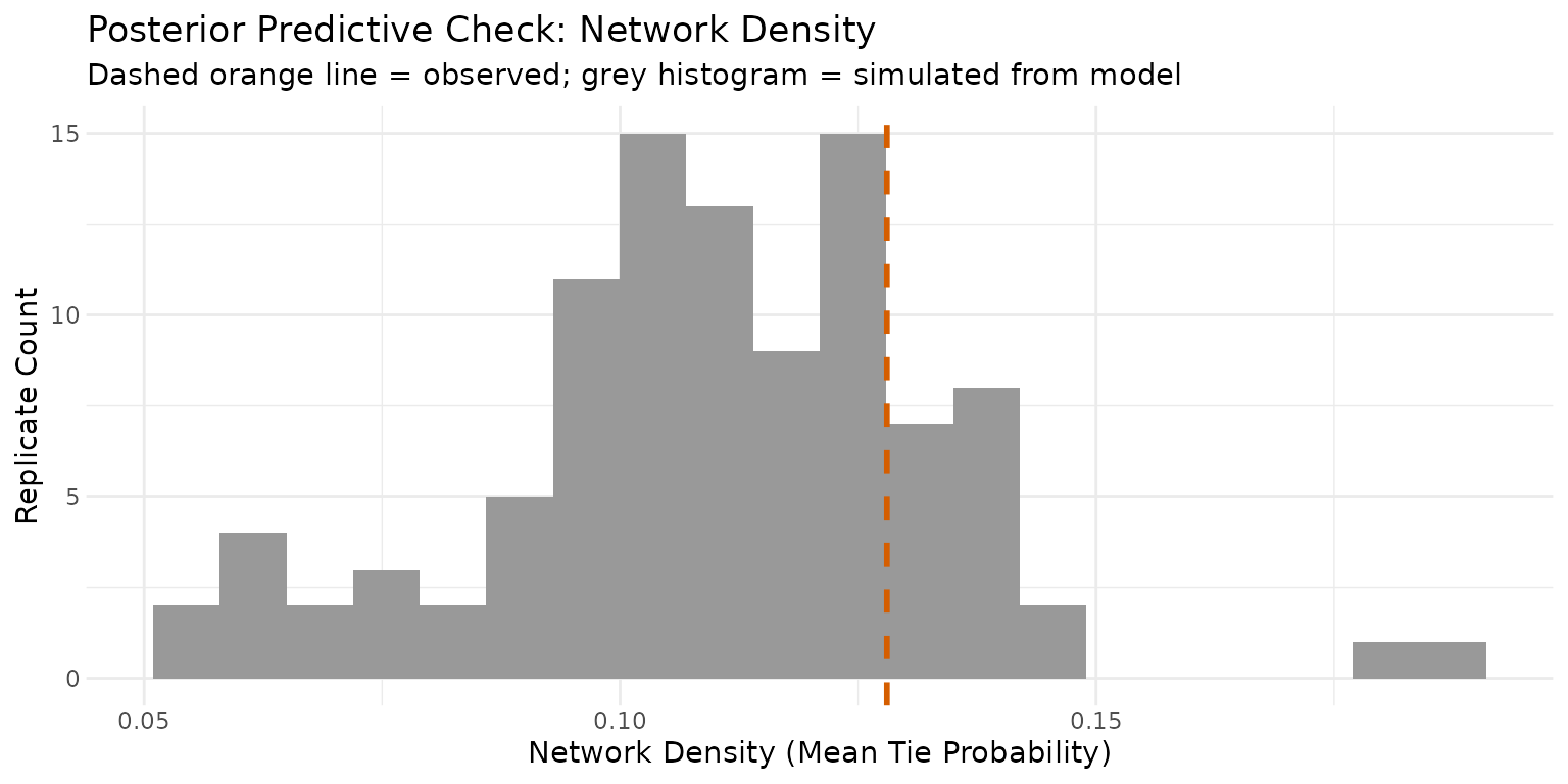

Practical Tips

Choosing R (latent dimensions). Start with R = 0 (no latent space), then try R = 1 and R = 2 and compare GOF. ame() / lame() warn when R > floor(n/3) because at that rank the multiplicative effects absorb structure that belongs to the additive effects; in practice R = 2 or R = 3 is the right default.

MCMC settings. For exploratory work, burn = 500, nscan = 2000, odens = 25 is fine. For a final run, use at least burn = 2000, nscan = 10000, odens = 25 and check convergence with trace_plot().

Variance components. Include rvar = TRUE and cvar = TRUE unless you have a specific reason not to. Include dcor = TRUE for directed networks where reciprocity is plausible.

What’s Next?

• Multiple time periods? See the lame overview for longitudinal models
• Two types of nodes? See the bipartite vignette
• Evolving network structure? See the dynamic effects vignette
• Other data types? See ?ame for the supported family options

References

Hoff, PD (2021). Additive and Multiplicative Effects Network Models. Statistical Science 36, 34–50.

Minhas, S., Dorff, C., Gallop, M. B., Foster, M., Liu, H., Tellez, J., & Ward, M. D. (2022). Taking dyads seriously. Political Science Research and Methods, 10(4), 703–721.